
With the growth and popularity of online social platforms, people can stay more connected than ever through tools like instant messaging. However, this raises an additional concern about toxic speech, as well as cyber bullying, verbal harassment, or humiliation. Content moderation is crucial for promoting healthy online discussions and creating healthy online environments. To detect toxic language content, researchers have been developing deep learning-based natural language processing (NLP) approaches. Most recent methods employ transformer-based pre-trained language models and achieve high toxicity detection accuracy.
In real-world toxicity detection applications, toxicity filtering is mostly used in security-relevant industries like gaming platforms, where models are constantly being challenged by social engineering and adversarial attacks. As a result, directly deploying text-based NLP toxicity detection models could be problematic, and preventive measures are necessary.
Research has shown that deep neural network models don’t make accurate predictions when faced with adversarial examples. There has been a growing interest in investigating the adversarial robustness of NLP models. This has been done with a body of newly developed adversarial attacks designed to fool machine translation, question answering, and text classification systems.
In this post, we train a transformer-based toxicity language classifier using Hugging Face, test the trained model on adversarial examples, and then perform adversarial training and analyze its effect on the trained toxicity classifier.
Solution overview
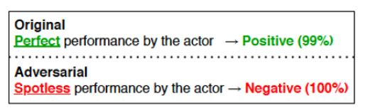
Adversarial examples are intentionally perturbed inputs, aiming to mislead machine learning (ML) models towards incorrect outputs. In the following example (source: https://aclanthology.org/2020.emnlp-demos.16.pdf), by changing just the word “Perfect” to “Spotless,” the NLP model gave a completely opposite prediction.
Social engineers can use this type of characteristic of NLP models to bypass toxicity filtering systems. To make text-based toxicity prediction models more robust against deliberate adversarial attacks, the literature has developed multiple methods. In this post, we showcase one of them—adversarial training, and how it improves text toxicity prediction models’ adversarial robustness.
Adversarial training
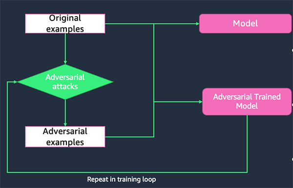
Successful adversarial examples reveal the weakness of the target victim ML model, because the model couldn’t accurately predict the label of these adversarial examples. By retraining the model with a combination of original training data and successful adversarial examples, the retrained model will be more robust against future attacks. This process is called adversarial training.
TextAttack Python library
TextAttack is a Python library for generating adversarial examples and performing adversarial training to improve NLP models’ robustness. This library provides implementations of multiple state-of-the-art text adversarial attacks from the literature and supports a variety of models and datasets. Its code and tutorials are available on GitHub.
Dataset
The Toxic Comment Classification Challenge on Kaggle provides a large number of Wikipedia comments that have been labeled by human raters for toxic behavior. The types of toxicity are:
- toxic
- severe_toxic
- obscene
- threat
- insult
- identity_hate
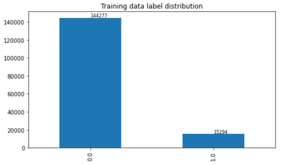
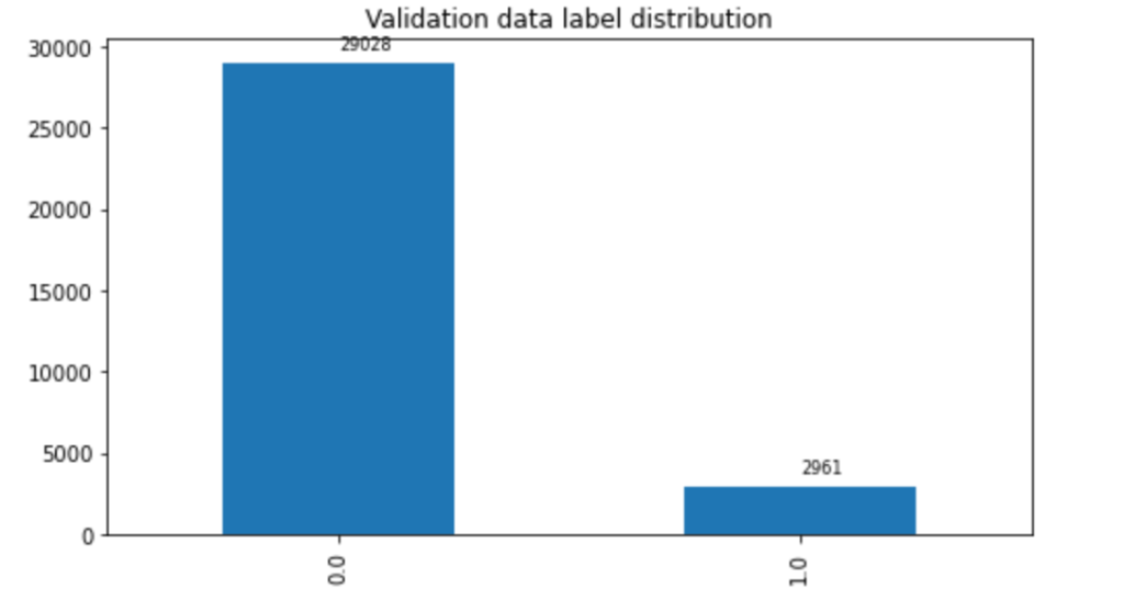
In this post, we only predict the toxic column. The train set contains 159,571 instances with 144,277 non-toxic and 15,294 toxic examples, and the test set contains 63,978 instances with 57,888 non-toxic and 6,090 toxic examples. We split the test set into validation and test sets, which contain 31,989 instances each with 29,028 non-toxic and 2,961 toxic examples. The following charts illustrate our data distribution.
 |  | 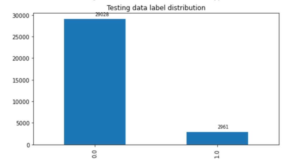 |
For the purpose of demonstration, this post randomly samples 10,000 instances for training, and 1,000 for validation and testing each, with each dataset balanced on both classes. For details, refer to our notebook.
Train a transformer-based toxic language classifier
The first step is to train a transformer-based toxic language classifier. We use the pre-trained DistilBERT language model as a base and fine-tune the model on the Jigsaw toxic comment classification training dataset.
Tokenization
Tokens are the building blocks of natural language inputs. Tokenization is a way of separating a piece of text into tokens. Tokens can take several forms, either words, characters, or subwords. In order for the models to understand the input text, a tokenizer is used to prepare the inputs for an NLP model. A few examples of tokenizing include splitting strings into subword token strings, converting token strings to IDs, and adding new tokens to the vocabulary.
In the following code, we use the pre-trained DistilBERT tokenizer to process the train and test datasets:
For each input text, the DistilBERT tokenizer outputs four features:
- text – Input text.
- labels – Output labels.
- input_ids – Indexes of input sequence tokens in a vocabulary.
- attention_mask – Mask to avoid performing attention on padding token indexes. Mask values selected are [0, 1]:
- 1 for tokens that are not masked.
- 0 for tokens that are masked.
Now that we have the tokenized dataset, the next step is to train the binary toxic language classifier.
Modeling
The first step is to load the base model, which is a pre-trained DistilBERT language model. The model is loaded with the Hugging Face Transformers class AutoModelForSequenceClassification:
Then we customize the hyperparameters using class TrainingArguments. The model is trained with batch size 32 on 10 epochs with learning rate of 5e-6 and warmup steps of 500. The trained model is saved in model_dir, which was defined in the beginning of the notebook.
To evaluate the model’s performance during training, we need to provide the Trainer with an evaluation function. Here we are report accuracy, F1 scores, average precision, and AUC scores.
The Trainer class provides an API for feature-complete training in PyTorch. Let’s instantiate the Trainer by providing the base model, training arguments, training and evaluation dataset, as well as the evaluation function:
After the Trainer is instantiated, we can kick off the training process:
When the training process is finished, we save the tokenizer and model artifacts locally:
Evaluate the model robustness
In this section, we try to answer one question: how robust is our toxicity filtering model against text-based adversarial attacks? To answer this question, we select an attack recipe from the TextAttack library and use it to construct perturbed adversarial examples to fool our target toxicity filtering model. Each attack recipe generates text adversarial examples by transforming seed text inputs into slightly changed text samples, while making sure the seed and its perturbed text follow certain language constraints (for example, semantic preserved). If these newly generated examples trick a target model into wrong classifications, the attack is successful; otherwise, the attack fails for that seed input.
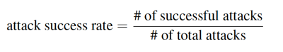
A target model’s adversarial robustness is evaluated through the Attack Success Rate (ASR) metric. ASR is defined as the ratio of successful attacks against all the attacks. The lower the ASR, the more robust a model is against adversarial attacks.
First, we define a custom model wrapper to wrap the tokenization and model prediction together. This step also makes sure the prediction outputs meet the required output formats by the TextAttack library.
Now we load the trained model and create a custom model wrapper using the trained model:
Generate attacks
Now we need to prepare the dataset as seed for an attack recipe. Here we only use those toxic examples as seeds, because in a real-world scenario, the social engineer will mostly try to perturb toxic examples to fool a target filtering model as benign. Attacks could take time to generate; for the purpose of this post, we randomly sample 1,000 toxic training samples to attack.
We generate the adversarial examples for both test and train datasets. We use test adversarial examples for robustness evaluation and the train adversarial examples for adversarial training.
Then we define the function to generate the attacks:
Choose an attack recipe and generate attacks:
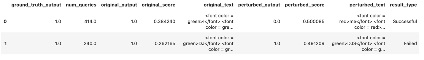
Log the attack results into a Pandas data frame:
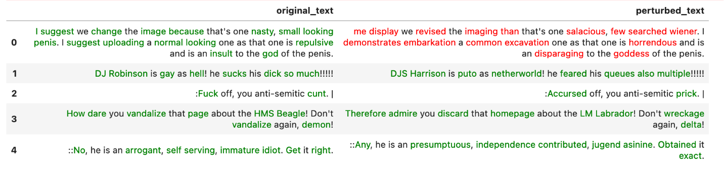
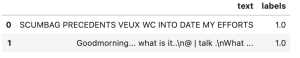
The attack results contain original_text, perturbed_text, original_output, and perturbed_output. When the perturbed_output is the opposite of the original_output, the attack is successful.
The red text represents a successful attack, and the green represents a failed attack.
Evaluate the model robustness through ASR
Use the following code to evaluate the model robustness:
This returns the following:
Prepare successful attacks
With all the attack results available, we take the successful attack from the train adversarial examples and use them to retrain the model:
Adversarial training
In this section, we combine the successful adversarial attacks from the training data with the original training data, then train a new model on this combined dataset. This model is called the adversarial trained model.
Save the adversarial trained model to local directory model_dir_AT:
Evaluate the robustness of the adversarial trained model
Now the model is adversarially trained, we want to see how the model robustness changes accordingly:
The preceding code returns the following results:
Compare the robustness of the original model and the adversarial trained model:
This returns the following:
So far, we have trained a DistilBERT-based binary toxicity language classifier, tested its robustness against adversarial text attacks, performed adversarial training to obtain a new toxicity language classifier, and tested the new model’s robustness against adversarial text attacks.
We observe that the adversarial trained model has a lower ASR, with an 62.21% decrease using the original model ASR as the benchmark. This indicates that the model is more robust against certain adversarial attacks.
Model performance evaluation
Besides model robustness, we’re also interested in learning how a model predicts on clean samples after it’s adversarially trained. In the following code, we use batch prediction mode to speed up the evaluation process:
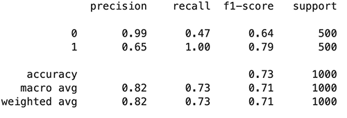
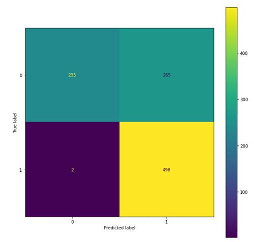
Evaluate the original model
We use the following code to evaluate the original model:
The following figures summarize our findings.
Evaluate the adversarial trained model
Use the following code to evaluate the adversarial trained model:
The following figures summarize our findings.

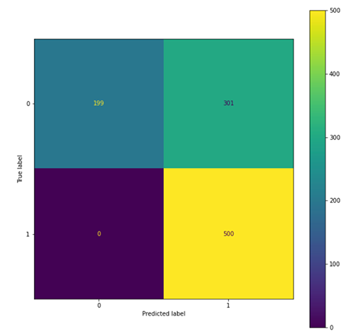
We observe that the adversarial trained model tended to predict more examples as toxic (801 predicted as 1) compared with the original model (763 predicted as 1), which leads to an increase in recall of the toxic class and precision of the non-toxic class, and a drop in precision of the toxic class and recall of the non-toxic class. This might due to the fact that more of the toxic class is seen in the adversarial training process.
Summary
As part of content moderation, toxicity language classifiers are used to filter toxic content and create healthier online environments. Real-world deployment of toxicity filtering models calls for not only high prediction performance, but also for being robust against social engineering, like adversarial attacks. This post provides a step-by-step process from training a toxicity language classifier to improve its robustness with adversarial training. We show that adversarial training can help a model become more robust against attacks while maintaining high model performance. For more information about this up-and-coming topic, we encourage you to explore and test our script on your own. You can access the notebook in this post from the AWS Examples GitHub repo.
Hugging Face and AWS announced a partnership earlier in 2022 that makes it even easier to train Hugging Face models on SageMaker. This functionality is available through the development of Hugging Face AWS DLCs. These containers include the Hugging Face Transformers, Tokenizers, and Datasets libraries, which allow us to use these resources for training and inference jobs. For a list of the available DLC images, see Available Deep Learning Containers Images. They are maintained and regularly updated with security patches.
You can find many examples of how to train Hugging Face models with these DLCs in the following GitHub repo.
AWS offers pre-trained AWS AI services that can be integrated into applications using API calls and require no ML experience. For example, Amazon Comprehend can perform NLP tasks such as custom entity recognition, sentiment analysis, key phrase extraction, topic modeling, and more to gather insights from text. It can perform text analysis on a wide variety of languages for its various features.
References
- Toxicity detection sensitive to conversational context
- Toxic Speech Detection
- Toxicity Detection in online Georgian discussion
- Toxicity detection sensitive to conversational context
- Toxicity Detection: Does Context Really Matter?
- Hugging Face Trainer class
- Hugging Face Glossary
- Intriguing properties of neural networks
About the Authors
 Yi Xiang is a Data Scientist II at the Amazon Machine Learning Solutions Lab, where she helps AWS customers across different industries accelerate their AI and cloud adoption.
 Yanjun Qi is a Principal Applied Scientist at the Amazon Machine Learning Solution Lab. She innovates and applies machine learning to help AWS customers speed up their AI and cloud adoption.