Differential privacy (DP) is a rigorous mathematical definition of privacy. DP algorithms are randomized to protect user data by ensuring that the probability of any particular output is nearly unchanged when a data point is added or removed. Therefore, the output of a DP algorithm does not disclose the presence of any one data point. There has been significant progress in both foundational research and adoption of differential privacy with contributions such as the Privacy Sandbox and Google Open Source Library.
ML and data analytics algorithms can often be described as performing multiple basic computation steps on the same dataset. When each such step is differentially private, so is the output, but with multiple steps the overall privacy guarantee deteriorates, a phenomenon known as the cost of composition. Composition theorems bound the increase in privacy loss with the number k of computations: In the general case, the privacy loss increases with the square root of k. This means that we need much stricter privacy guarantees for each step in order to meet our overall privacy guarantee goal. But in that case, we lose utility. One way to improve the privacy vs. utility trade-off is to identify when the use cases admit a tighter privacy analysis than what follows from composition theorems.
Good candidates for such improvement are when each step is applied to a disjoint part (slice) of the dataset. When the slices are selected in a data-independent way, each point affects only one of the k outputs and the privacy guarantees do not deteriorate with k. However, there are applications in which we need to select the slices adaptively (that is, in a way that depends on the output of prior steps). In these cases, a change of a single data point may cascade — changing multiple slices and thus increasing composition cost.
In “Õptimal Differentially Private Learning of Thresholds and Quasi-Concave Optimization”, presented at STOC 2023, we describe a new paradigm that allows for slices to be selected adaptively and yet avoids composition cost. We show that DP algorithms for multiple fundamental aggregation and learning tasks can be expressed in this Reorder-Slice-Compute (RSC) paradigm, gaining significant improvements in utility.
The Reorder-Slice-Compute (RSC) paradigm
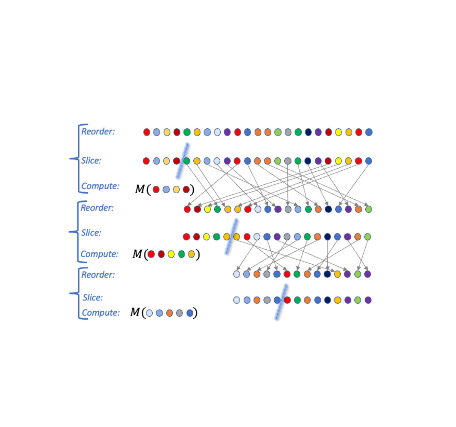
An algorithm A falls in the RSC paradigm if it can be expressed in the following general form (see visualization below). The input is a sensitive set D of data points. The algorithm then performs a sequence of k steps as follows:
- Select an ordering over data points, a slice size m, and a DP algorithm M. The selection may depend on the output of A in prior steps (and hence is adaptive).
- Slice out the (approximately) top m data points according to the order from the dataset D, apply M to the slice, and output the result.
 |
| A visualization of three Reorder-Slice-Compute (RSC) steps. |
If we analyze the overall privacy loss of an RSC algorithm using DP composition theorems, the privacy guarantee suffers from the expected composition cost, i.e., it deteriorates with the square root of the number of steps k. To eliminate this composition cost, we provide a novel analysis that removes the dependence on k altogether: the overall privacy guarantee is close to that of a single step! The idea behind our tighter analysis is a novel technique that limits the potential cascade of affected steps when a single data point is modified (details in the paper).
Tighter privacy analysis means better utility. The effectiveness of DP algorithms is often stated in terms of the smallest input size (number of data points) that suffices in order to release a correct result that meets the privacy requirements. We describe several problems with algorithms that can be expressed in the RSC paradigm and for which our tighter analysis improved utility.
Private interval point
We start with the following basic aggregation task. The input is a dataset D of n points from an ordered domain X (think of the domain as the natural numbers between 1 and |X|). The goal is to return a point y in X that is in the interval of D, that is between the minimum and the maximum points in D.
The solution to the interval point problem is trivial without the privacy requirement: simply return any point in the dataset D. But this solution is not privacy-preserving as it discloses the presence of a particular datapoint in the input. We can also see that if there is only one point in the dataset, a privacy-preserving solution is not possible, as it must return that point. We can therefore ask the following fundamental question: What is the smallest input size N for which we can solve the private interval point problem?
It is known that N must increase with the domain size |X| and that this dependence is at least the iterated log function log* |X| [1, 2]. On the other hand, the best prior DP algorithm required the input size to be at least (log* |X|)1.5. To close this gap, we designed an RSC algorithm that requires only an order of log* |X| points.
The iterated log function is extremely slow growing: It is the number of times we need to take a logarithm of a value before we reach a value that is equal to or smaller than 1. How did this function naturally come out in the analysis? Each step of the RSC algorithm remapped the domain to a logarithm of its prior size. Therefore there were log* |X| steps in total. The tighter RSC analysis eliminated a square root of the number of steps from the required input size.
Even though the interval point task seems very basic, it captures the essence of the difficulty of private solutions for common aggregation tasks. We next describe two of these tasks and express the required input size to these tasks in terms of N.
Private approximate median
One of these common aggregation tasks is approximate median: The input is a dataset D of n points from an ordered domain X. The goal is to return a point y that is between the ⅓ and ⅔ quantiles of D. That is, at least a third of the points in D are smaller or equal to y and at least a third of the points are larger or equal to y. Note that returning an exact median is not possible with differential privacy, since it discloses the presence of a datapoint. Hence we consider the relaxed requirement of an approximate median (shown below).
We can compute an approximate median by finding an interval point: We slice out the N smallest points and the N largest points and then compute an interval point of the remaining points. The latter must be an approximate median. This works when the dataset size is at least 3N.
 |
| An example of a data D over domain X, the set of interval points, and the set of approximate medians. |
Private learning of axis-aligned rectangles
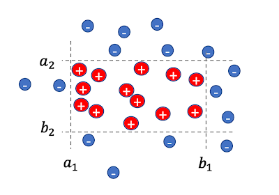
For the next task, the input is a set of n labeled data points, where each point x = (x1,….,xd) is a d-dimensional vector over a domain X. Displayed below, the goal is to learn values ai , bi for the axes i=1,…,d that define a d-dimensional rectangle, so that for each example x
- If x is positively labeled (shown as red plus signs below) then it lies within the rectangle, that is, for all axes i, xi is in the interval [ai ,bi], and
- If x is negatively labeled (shown as blue minus signs below) then it lies outside the rectangle, that is, for at least one axis i, xi is outside the interval [ai ,bi].
 |
| A set of 2-dimensional labeled points and a respective rectangle. |
Any DP solution for this problem must be approximate in that the learned rectangle must be allowed to mislabel some data points, with some positively labeled points outside the rectangle or negatively labeled points inside it. This is because an exact solution could be very sensitive to the presence of a particular data point and would not be private. The goal is a DP solution that keeps this necessary number of mislabeled points small.
We first consider the one-dimensional case (d = 1). We are looking for an interval [a,b] that covers all positive points and none of the negative points. We show that we can do this with at most 2N mislabeled points. We focus on the positively labeled points. In the first RSC step we slice out the N smallest points and compute a private interval point as a. We then slice out the N largest points and compute a private interval point as b. The solution [a,b] correctly labels all negatively labeled points and mislabels at most 2N of the positively labeled points. Thus, at most ~2N points are mislabeled in total.
 |
| Illustration for d = 1, we slice out N left positive points and compute an interval point a, slice out N right positive points and compute an interval point b. |
With d > 1, we iterate over the axes i = 1,….,d and apply the above for the ith coordinates of input points to obtain the values ai , bi . In each iteration, we perform two RSC steps and slice out 2N positively labeled points. In total, we slice out 2dN points and all remaining points were correctly labeled. That is, all negatively-labeled points are outside the final d-dimensional rectangle and all positively-labeled points, except perhaps ~2dN, lie inside the rectangle. Note that this algorithm uses the full flexibility of RSC in that the points are ordered differently by each axis. Since we perform d steps, the RSC analysis shaves off a factor of square root of d from the number of mislabeled points.
Training ML models with adaptive selection of training examples
The training efficiency or performance of ML models can sometimes be improved by selecting training examples in a way that depends on the current state of the model, e.g., self-paced curriculum learning or active learning.
The most common method for private training of ML models is DP-SGD, where noise is added to the gradient update from each minibatch of training examples. Privacy analysis with DP-SGD typically assumes that training examples are randomly partitioned into minibatches. But if we impose a data-dependent selection order on training examples, and further modify the selection criteria k times during training, then analysis through DP composition results in deterioration of the privacy guarantees of a magnitude equal to the square root of k.
Fortunately, example selection with DP-SGD can be naturally expressed in the RSC paradigm: each selection criteria reorders the training examples and each minibatch is a slice (for which we compute a noisy gradient). With RSC analysis, there is no privacy deterioration with k, which brings DP-SGD training with example selection into the practical domain.
Conclusion
The RSC paradigm was introduced in order to tackle an open problem that is primarily of theoretical significance, but turns out to be a versatile tool with the potential to enhance data efficiency in production environments.
Acknowledgments
The work described here was done jointly with Xin Lyu, Jelani Nelson, and Tamas Sarlos.

