Dynamically Splitting Wide Partitions in Cassandra for Time Series Workloads

By Rajiv Shringi, Kaidan Fullerton, Oleksii Tkachuk and Kartik Sathyanarayanan

Introduction

Netflix’s TimeSeries Abstraction is a scalable system for ingesting and querying petabytes of temporal event data with millisecond latency. We use Apache Cassandra 4.x as the underlying storage for these main reasons:

Throughput, latency, and cost: Cassandra can handle millions of low‑latency reads and writes in a cost-effective manner.
Operational maturity: Our data platform team has deep operational expertise running large Cassandra clusters in production.

However, using Cassandra at this scale introduces trade‑offs for TimeSeries workloads. A key challenge is wide partitions, as TimeSeries dataset partitions can grow quite large with events accumulating over time.

This problem is further compounded by the fact that TimeSeries servers routinely deal with a very high read throughput:

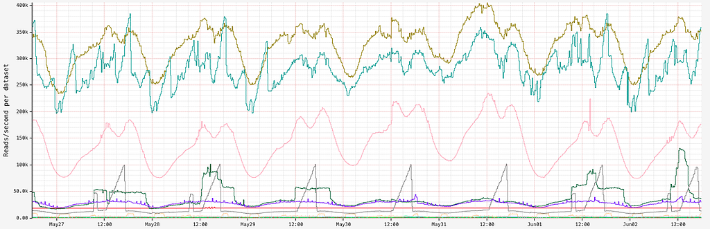
This post walks through our journey to reduce the impact of wide partitions in our TimeSeries datasets, the solutions we built, and the lessons we learned.

Impact of Wide Partitions

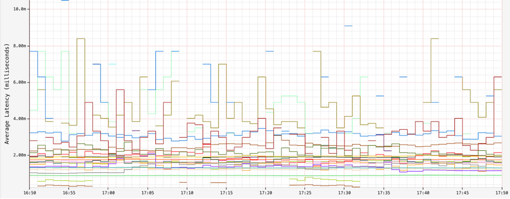
For most of our datasets, we observe an average read latency in the order of single-digit milliseconds:

However, in some datasets, as partitions grow too wide, we observe high read latencies in the order of seconds, especially towards the tail end:

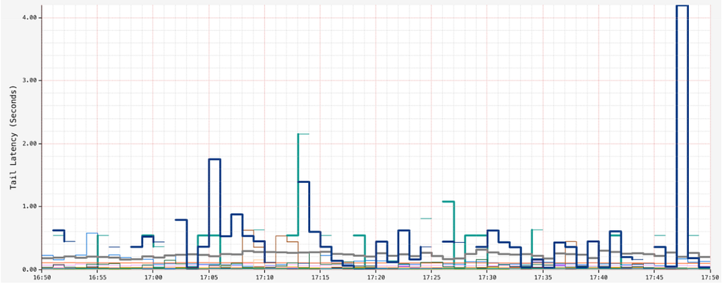
This can result in timeouts:

In extreme cases, if most of the reads target wide partitions, we can see Garbage Collection pauses, high CPU utilization and thread queueing.

High CPU utilization and thread-queueing in Cassandra clusters

Scaling up the underlying Cassandra cluster is always an option, but we need smarter alternatives than just throwing more money at the problem.

TimeSeries Partitioning Strategy

The TimeSeries Abstraction was designed to solve the problem of wide partitions by dividing the data into discrete time chunks. For more in-depth information, refer to our previous blog.

To summarize, here is an illustration of how TimeSeries partitioning strategy helps us break up wide partitions into manageable chunks.

Time Series partitioning breaking up a dataset into Time slices, time buckets and event buckets

This strategy further allows us to efficiently query and drop data based on time, without having to deal with tombstones.

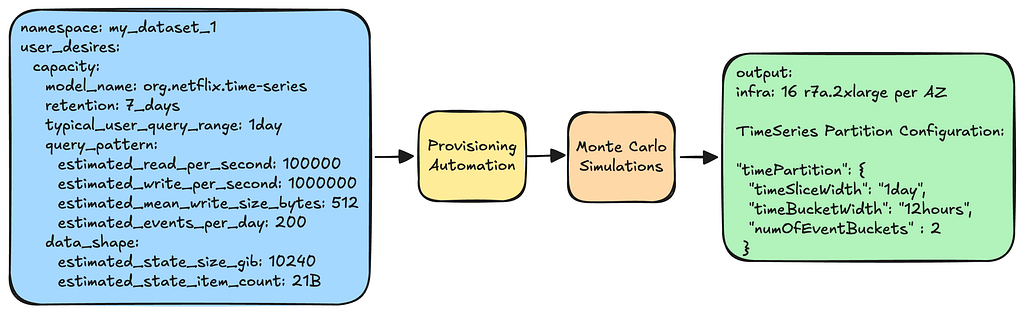
Picking the Partitioning Strategy

When a namespace (a.k.a. dataset) is created, users must specify their anticipated workload characteristics. This specification is then fed into our provisioning pipeline. The pipeline processes these inputs, runs Monte Carlo simulations, and produces an optimal infrastructure and partition configuration.

Provisioning picks optimal infra and configuration based on user inputs

You can learn more about our methodology of capacity planning in this insightful AWS re:Invent talk given by one of our stunning colleagues.

The Problem with the Current Approach

Although this method of provisioning is effective in many situations, it proves insufficient for TimeSeries workloads under these conditions:

Workload is unknown or inaccurately estimated: Early on in a project, users can lack a reliable picture of production traffic or simply misestimate key parameters.
Workload evolves over time: Traffic patterns, client behavior, and product requirements change. A “good” partitioning strategy on day one can become inefficient months later.
Data outliers exist: Not all TimeSeries IDs behave the same. A small percentage of IDs can receive a vastly higher volume of events than the rest.

Fortunately, our design with discrete Time Slices gives us a natural escape hatch for the first two scenarios; each new Time Slice can use a different partitioning strategy.

Each Time Slice can have a unique partition strategy

However, manually adjusting these configurations in a fleet that has thousands of TimeSeries datasets is not sustainable. We need automation.

Solution 1: Time Slice Re-Partitioning

Cassandra exposes useful introspection APIs for understanding data usage and access patterns. For example, nodetool tablehistograms provide percentile distributions for partition sizes in a table. Using these tools, we can detect cases of both over and under partitioning.

Below is an example of over‑partitioning, where the TimeSeries provisioning pipeline selected very small time_bucket intervals based on user provided inputs:

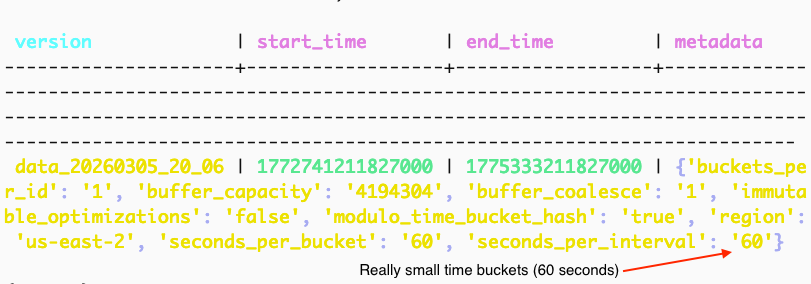
Provisioning selected 60s time buckets based on user inputs

causing partitions to have less than 10 KB of data, leading to high read amplification and thread queueing:

Histogram of the given Cassandra table showing partition size percentiles

In order to tune partition strategies efficiently, we added a background worker, which monitors partition histograms of Time Slices attached to a given application, and exposes it via a Cassandra virtual table:

Histograms exposed through a Cassandra Virtual table

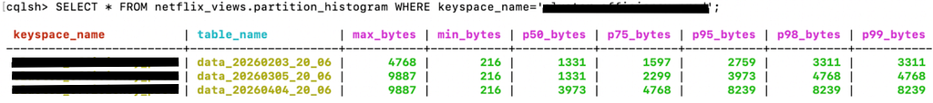
It then computes an adjustment factor when it detects partition sizes not meeting a configured density. This configured density is often set between 2 MiB to 10 MiB depending on the workload.

DynamicTimeSliceConfigWorker: 
namespace: my_dataset_1
Observed: TimeSlices have p99 partitions below configured target of 10MB. 
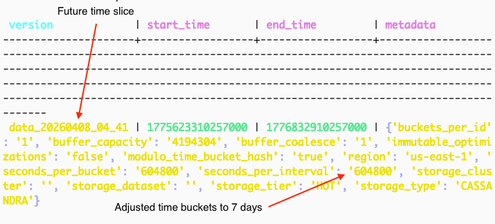
Proposed: time_bucket interval: 60s -> 604800s

The worker can then update future Time Slices with the new partition strategy:

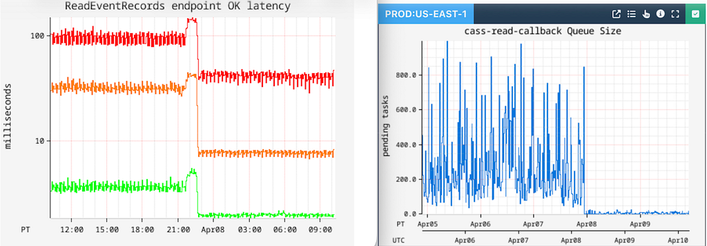
Partitioning adjusted for future Time Slice(s)

This strategy has yielded real results in reducing our read latencies, as well as reducing the number of timeouts caused by thread queueing.

Reduction in tail latency and thread queueing for

However, this strategy only works if most of the data exhibits such behavior that warrants re-partitioning of the entire table. It does not work in cases where only a percentage of IDs within the table are wide.

We have a couple of options here:

Do Nothing: This is sometimes the right approach if there is no observed impact to the application’s top-level metrics.
Partial Returns: We implemented a ‘Partial Return’ feature, which aborts an inflight request if it has breached a configured latency SLO, while returning whatever data it has collected up until that point. This is a great option for clients who care more about latency than fetching all the data.

Tail latency drops around the SLO cutoff as Partial Returns are enabled

Block IDs: This is an extreme step but worth mentioning, because we do deal with bad data that occasionally seeps into the system e.g. test or spam IDs that can make the system unstable.

dgwts.config.<dataset>.block.Ids: "<tsid-1>, <tsid-2>, <tsid-3>"

Ultimately, we encounter scenarios where valid and important TimeSeries IDs accumulate a high enough volume of events, with callers needing to process all the related data. Simply tolerating elevated latencies or timeouts when querying these IDs is not a desirable outcome.

This is where dynamic partitioning comes into play.

Solution 2: Dynamic Partitioning per ID

Dynamic partitioning is an asynchronous pipeline that auto-detects and splits wide partitions on a TimeSeries ID level rather than at the table level.

It has three main stages:

Detection: Detects wide partitions for a given TimeSeries ID during the read path.
Planning & Splitting: Plans and executes splits of those partitions into optimal sizes asynchronously.
Serving Reads: Re-routes the read queries transparently to read data from the split partitions when ready.

This is how it works at a high level; we will dive into details after:

Dynamic Wide Partition Split Async Pipeline

Here are the different stages of the pipeline:

Detection

Every TimeSeries read operation tracks how many bytes are read for a given partition. If the bytes read exceed a configured threshold, the server emits a detection event to Kafka:

{
  "time_slice": "data_20260328", // the Cassandra table this event was detected in
  "time_series_id": "profileId:123", // the ID detected as wide
  "time_bucket": 7, // the existing time_bucket partition
  "event_bucket": 2, // the existing event_bucket partition
  "immutable": true, // TimeSeries servers can compute if this partition is no longer receiving writes
  "version": "0" // reserved for future use e.g. invalidate if partition is no longer immutable
}

Our decision to detect wide partitions on reads, as opposed to writes, is based on our observation that the majority of the data in the wild doesn’t need this treatment. The slight downside is that some reads on these large partitions may suffer sub-optimal performance for a very short duration (typically seconds) until this process catches up.

Immutability

Although splitting mutable partitions is possible, it is inherently more complex. As a first step towards solving this problem, we chose to reduce the surface area of this change by focusing on immutable partitions, while still meaningfully reducing caller timeouts.

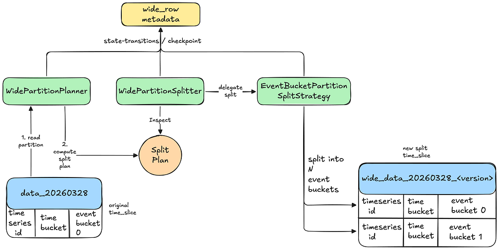
Planning

Detection may occur based on a partial read, so the planner must still read the entire partition once to compute an accurate split plan. The checkpointing becomes crucial here. For planning reads that fail to process the entire partition, the process can always continue from the last saved checkpoint.

Checkpointing

The wide_row metadata table serves as the backbone for state transitions and checkpointing of partition splits. It also stores information that is used later by TimeSeries servers to properly route Read queries.

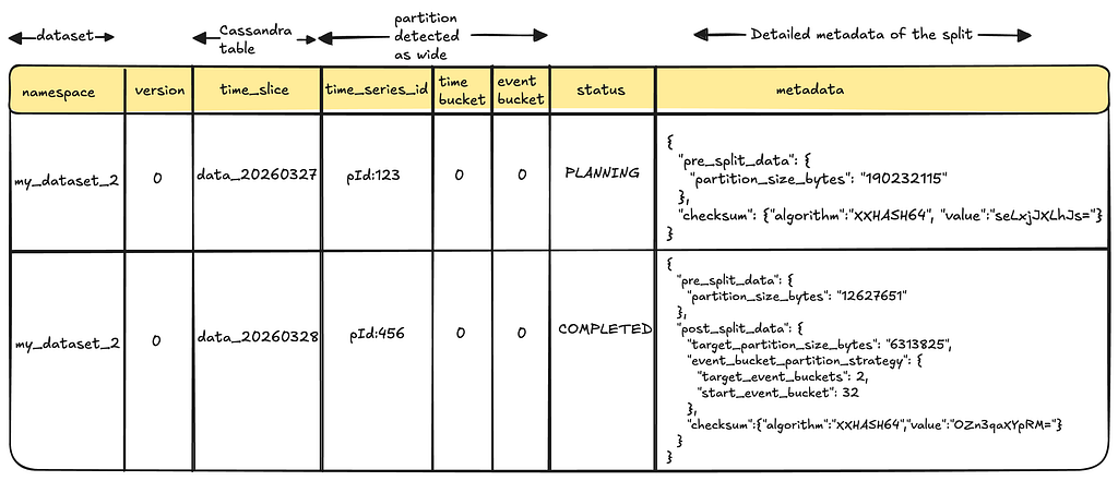
wide_row metadata for storing split states and checkpoints

Splitting

The Planner delegates the splitting of data to an appropriate split-strategy. For example, if EventBucketPartitionSplitStrategy is selected, we split the partition by assigning more event buckets to the same time bucket. If the partition is ultra-wide, we cap the number of event buckets we split into, in order to control the resultant read amplification. Spreading into multiple partitions in such cases is still beneficial in order to spread the read workload to multiple Cassandra replicas.

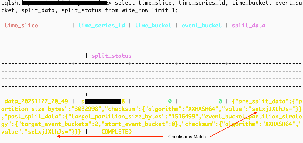
Split by assigning more event buckets for a given time bucket

Validating Splits

The Planner stores a pre-split checksum of a given partition during the planning phase, while the Splitter computes and stores the post-split checksum. The split status is marked as completed only if the two checksums match.

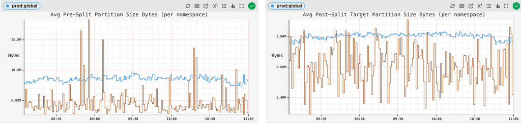
Ensure checksums match pre- and post-split before marking a split as COMPLETED

Tracking Splits

The pre- and post-split partition sizes across different datasets are tracked to see how effectively the partition splits are being planned and executed:

Track pre- and post-split partition sizes to ensure we are splitting optimally

Serving Reads

The TimeSeries servers load the partition-keys of completed splits periodically into in-memory Bloom filters. Every read operation checks the Bloom filter to see whether a query can be diverted to the split partitions.

Here is what the Read path looks like:

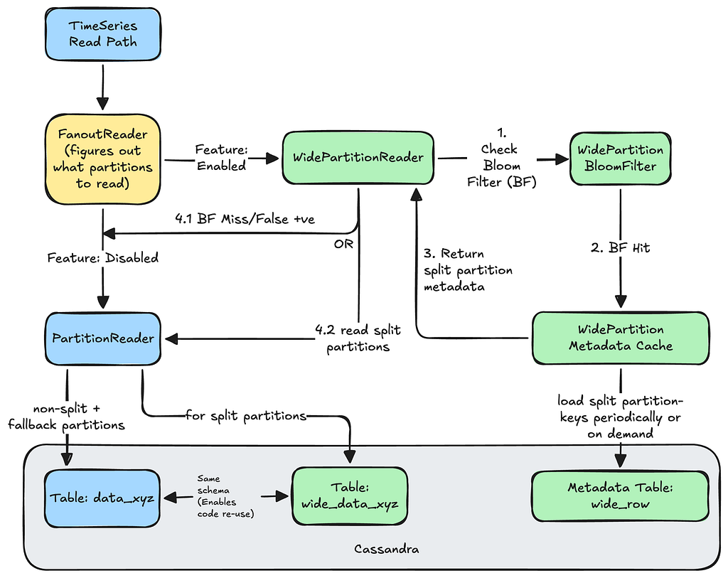
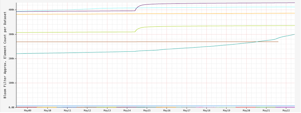
Read path for diverting reads to existing or split partitions

The size of the Bloom filters is monitored to ensure we have enough memory per server. Due to the compactness of partition keys, and ratio of wide partitions in a given dataset, the filters fit comfortably in each server instance.

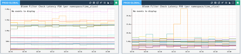
Bloom filter approximate element count per namespace and time slice

The Bloom filter latency to check whether a given partition key is wide for every read request is typically in single-digit microseconds or better, making this diversion practically invisible to the callers.

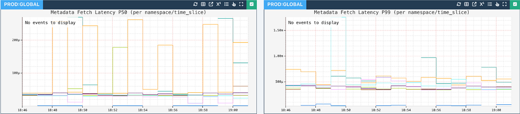
Latency for checking Bloom filters is extremely small for callers to notice the diversion

For the cases that do end up with a Bloom filter hit, the TimeSeries servers lookup the wide_row metadata to see how to read a specific wide partition:

{
  "pre_split_data": {
    "time_slice": "data_20260328",
    "time_series_id": "6313825", → What to read
    "time_bucket": 0,
    "event_bucket": 2
    …
  },
  "post_split_data": {
    "time_slice": "wide_data_20260328_0", → Where to read it from
    "event_bucket_partition_strategy": { → Strategy to delegate to for reading
    "target_event_buckets": 2,
    "start_event_bucket": 32 → How should the strategy read it
  }
  …
}

This metadata read is backed by a read-through cache, making it quite performant:

Metadata fetch latency is quite low to affect read operations

Finally, the reads for the split partitions are delegated to our existing PartitionReader. Having the same schema for the split table allows us to reuse code and minimize changes.

Fallbacks

The existing wide partition from the original time slice is never deleted. This helps us in creating safe fallbacks in many different scenarios of partial failures and eventual consistency. The slightly larger storage space we use as a result is worth the operational safety we gain.

Building Additional Confidence

Serving incorrect reads would be disastrous. To establish trust beyond checksums, we leveraged additional mechanisms such as:

Using our existing Data Bridge pipelines to verify splits offline:

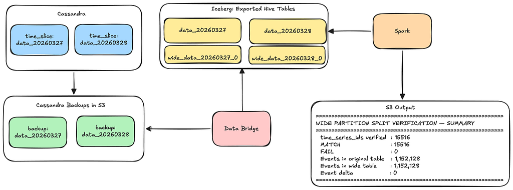
Spark job to ensure that the split data is an exact match to the original data

Implementing a phased rollout strategy to safely advance through stages as our confidence in the system grew:

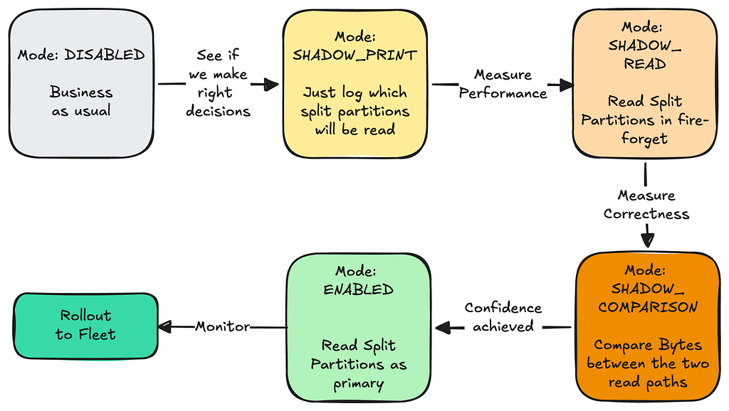
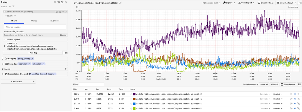
Advance through Read modes once previous mode passes checks

A critical part of this phased rollout was the Comparison phase, which compared bytes served by old read path and the new read path while in shadow mode:

A chart of bytes match vs bytes differ in a given shadow period

Results

As a result of these dynamic splits, we see a huge improvement in the average read latency of most wide partitions, bringing it down from seconds:

Existing average latency for reading wide partitions

to low double-digit milliseconds!

Average latency for reading dynamically split partitions

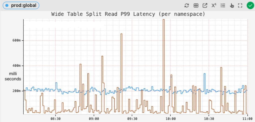
Tail latencies of reading wide partitions dropped from several seconds:

Existing tail latency for reading wide partitions

to around 200 ms or better:

Tail latency for reading dynamically split partitions

resulting in a drop in read timeouts:

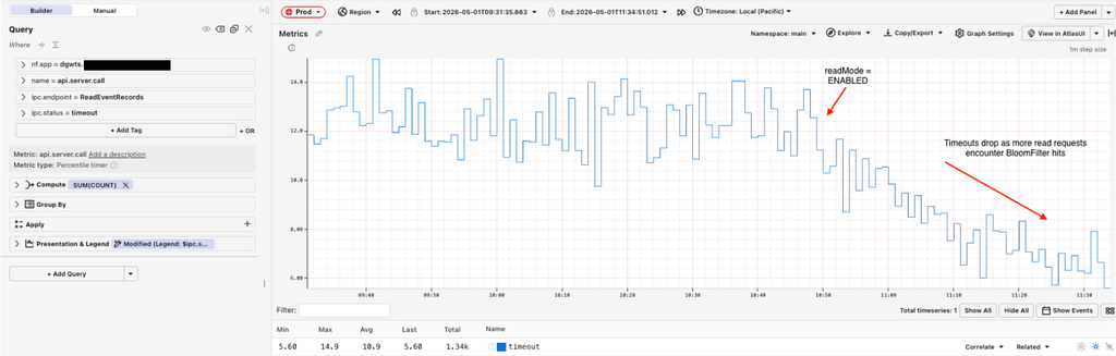
Further, for extreme wide rows, where a dataset would face constant timeouts and unavailability blips, the service was able to paginate and query 500MB+ partitions while remaining available:

grpc … com.netflix.dgw.ts.TimeSeriesService/SearchEventRecords -d
'{"namespace": "...",
    "search_query": {...},
    "time_interval": {
      "start": "2026–05–11T23:42:51.484398Z",
      "end": "2026–05–12T00:13:50.694205Z"
    },
    "pageSize" : 1000,
  }'
# Response:
{
  "next_page_token" : ….,
  "records": [
    {
      …
    }
  ],
  "response_context": [{
    "namespace": "...",
    …
    # Trades elevated latency for being available
    "time_taken": "41.072410142s"
    }
  ]
}

Conclusion

There is more work planned around this feature, like splitting mutable wide partitions, or re-processing previously failed splits, but this has been a successful start in improving service performance and reducing our support burden.

Further, we would like to highlight some key lessons that we learned at different points in this journey.

Reducing Surface Area: As a first step, explore simpler solutions that can still deliver meaningful impact. Also, reducing the surface area of a complex change and deploying incrementally pays off operationally.
Building Confidence: Invest time and resources to build confidence in new features, especially when justified by the feature complexity, deployment blast radius, and/or potential impact.

Acknowledgements: Special thanks to our stunning colleagues who further contributed to this feature’s success: Tom DeVoe, Chris Lohfink, Sumanth Pasupuleti and Joey Lynch.

Dynamically Splitting Wide Partitions in Cassandra for Time Series Workloads was originally published in Netflix TechBlog on Medium, where people are continuing the conversation by highlighting and responding to this story.