Hosting ML Models on Amazon SageMaker using Triton: XGBoost, LightGBM, and Treelite Models

One of the most popular models available today is XGBoost. With the ability to solve various problems such as classification and regression, XGBoost has become a popular option that also falls into the category of tree-based models. In this post, we dive deep to see how Amazon SageMaker can serve these models using NVIDIA Triton Inference Server. Real-time inference workloads can have varying levels of requirements and service level agreements (SLAs) in terms of latency and throughput, and can be met using SageMaker real-time endpoints.

SageMaker provides single model endpoints, which allow you to deploy a single machine learning (ML) model against a logical endpoint. For other use cases, you can choose to manage cost and performance using multi-model endpoints, which allow you to specify multiple models to host behind a logical endpoint. Regardless of the option the you choose, SageMaker endpoints allow a scalable mechanism for even the most demanding enterprise customers while providing value in a plethora of features, including shadow variants, auto scaling, and native integration with Amazon CloudWatch (for more information, refer to CloudWatch Metrics for Multi-Model Endpoint Deployments).

Triton supports various backends as engines to support the running and serving of various ML models for inference. For any Triton deployment, it’s crucial to know how the backend behavior impacts your workloads and what to expect so that you can be successful. In this post, we help you understand the Forest Inference Library (FIL) backend, which is supported by Triton on SageMaker, so that you can make an informed decision for your workloads and get the best performance and cost optimization possible.

Deep dive into the FIL backend

Triton supports the FIL backend to serve tree models, such as XGBoost, LightGBM, scikit-learn Random Forest, RAPIDS cuML Random Forest, and any other model supported by Treelite. These models have long been used for solving problems such as classification or regression. Although these types of models have traditionally run on CPUs, the popularity of these models and inference demands have led to various techniques to increase inference performance. The FIL backend utilizes many of these techniques by using cuML constructs and is built on C++ and the CUDA core library to optimize inference performance on GPU accelerators.

The FIL backend uses cuML’s libraries to use CPU or GPU cores to accelerate learning. In order to use these processors, data is referenced from host memory (for example, NumPy arrays) or GPU arrays (uDF, Numba, cuPY, or any library that supports the __cuda_array_interface__) API. After the data is staged in memory, the FIL backend can run processing across all the available CPU or GPU cores.

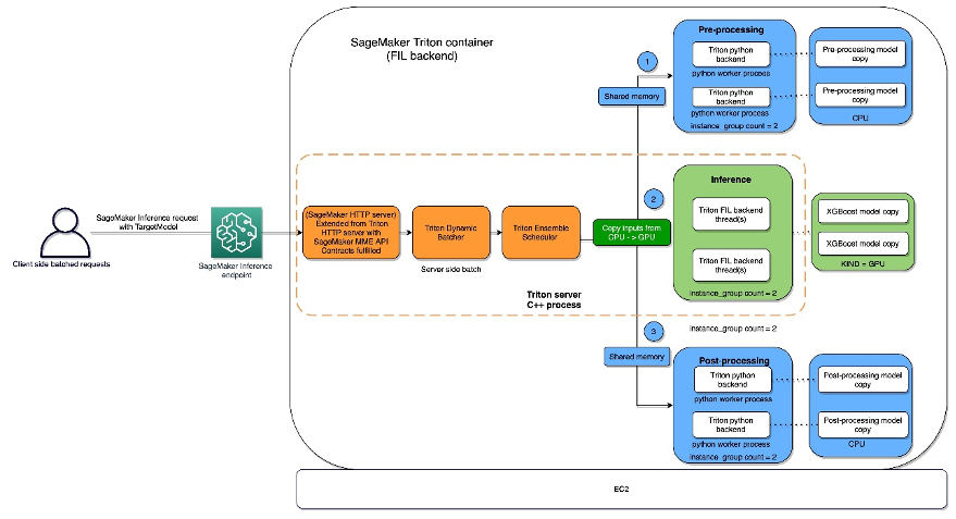
The FIL backend threads can communicate with each other without utilizing shared memory of the host, but in ensemble workloads, host memory should be considered. The following diagram shows an ensemble scheduler runtime architecture where you have the ability to fine-tune the memory areas, including CPU addressable shared memory that is used for inter-process communication between Triton (C++) and the Python process (Python backend) for exchanging tensors (input/output) with the FIL backend.

Triton Inference Server provides configurable options for developers to tune their workloads and optimize model performance. The configuration dynamic_batching allows Triton to hold client-side requests and batch them on the server side in order to efficiently use FIL’s parallel computation to inference the entire batch together. The option max_queue_delay_microseconds offers a fail-safe control of how long Triton waits to form a batch.

There are a number of other FIL-specific options available that impact performance and behavior. We suggest starting with storage_type. When running the backend on GPU, FIL creates a new memory/data structure that is a representation of the tree for which FIL can impact performance and footprint. This is configurable via the environment parameter storage_type, which has the options dense, sparse, and auto. Choosing the dense option will consume more GPU memory and doesn’t always result in better performance, so it’s best to check. In contrast, the sparse option will consume less GPU memory and can possibly perform as well or better than dense. Choosing auto will cause the model to default to dense unless doing so will consume significantly more GPU memory than sparse.

When it comes to model performance, you might consider emphasizing the threads_per_tree option. One thing that you may overserve in real-world scenarios is that threads_per_tree can have a bigger impact on throughput than any other parameter. Setting it to any power of 2 from 1–32 is legitimate. The optimal value is hard to predict for this parameter, but when the server is expected to deal with higher load or process larger batch sizes, it tends to benefit from a larger value than when it’s processing a few rows at a time.

Another parameter to be aware of is algo, which is also available if you’re running on GPU. This parameter determines the algorithm that’s used to process the inference requests. The options supported for this are ALGO_AUTO, NAIVE, TREE_REORG, and BATCH_TREE_REORG. These options determine how nodes within a tree are organized and can also result in performance gains. The ALGO_AUTO option defaults to NAIVE for sparse storage and BATCH_TREE_REORG for dense storage.

Lastly, FIL comes with Shapley explainer, which can be activated by using the treeshap_output parameter. However, you should keep in mind that Shapley outputs hurt performance due to its output size.

Model format

There is currently no standard file format to store forest-based models; every framework tends to define its own format. In order to support multiple input file formats, FIL imports data using the open-source Treelite library. This enables FIL to support models trained in popular frameworks, such as XGBoost and LightGBM. Note that the format of the model that you’re providing must be set in the model_type configuration value specified in the config.pbtxt file.

Config.pbtxt

Each model in a model repository must include a model configuration that provides the required and optional information about the model. Typically, this configuration is provided in a config.pbtxt file specified as ModelConfig protobuf. To learn more about the config settings, refer to Model Configuration. The following are some of the model configuration parameters:

• max_batch_size – This determines the maximum batch size that can be passed to this model. In general, the only limit on the size of batches passed to a FIL backend is the memory available with which to process them. For GPU runs, the available memory is determined by the size of Triton’s CUDA memory pool, which can be set via a command line argument when starting the server.
• input – Options in this section tell Triton the number of features to expect for each input sample.
• output – Options in this section tell Triton how many output values there will be for each sample. If the predict_proba option is set to true, then a probability value will be returned for each class. Otherwise, a single value will be returned, indicating the class predicted for the given sample.
• instance_group – This determines how many instances of this model will be created and whether they will use GPU or CPU.
• model_type – This string indicates what format the model is in (xgboost_json in this example, but xgboost, lightgbm, and tl_checkpoint are valid formats as well).
• predict_proba – If set to true, probability values will be returned for each class rather than just a class prediction.
• output_class – This is set to true for classification models and false for regression models.
• threshold – This is a score threshold for determining classification. When output_class is set to true, this must be provided, although it won’t be used if predict_proba is also set to true.
• storage_type – In general, using AUTO for this setting should meet most use cases. If AUTO storage is selected, FIL will load the model using either a sparse or dense representation based on the approximate size of the model. In some cases, you may want to explicitly set this to SPARSE in order to reduce the memory footprint of large models.

Triton Inference Server on SageMaker

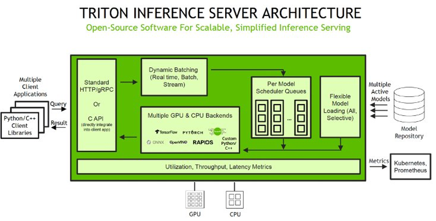
SageMaker allows you to deploy both single model and multi-model endpoints with NVIDIA Triton Inference Server. The following figure shows the Triton Inference Server high-level architecture. The model repository is a file system-based repository of the models that Triton will make available for inferencing. Inference requests arrive at the server and are routed to the appropriate per-model scheduler. Triton implements multiple scheduling and batching algorithms that can be configured on a model-by-model basis. Each model’s scheduler optionally performs batching of inference requests and then passes the requests to the backend corresponding to the model type. The backend performs inferencing using the inputs provided in the batched requests to produce the requested outputs. The outputs are then returned.

When configuring your auto scaling groups for SageMaker endpoints, you may want to consider SageMakerVariantInvocationsPerInstance as the primary criteria to determine the scaling characteristics of your auto scaling group. In addition, depending on whether your models are running on GPU or CPU, you may also consider using CPUUtilization or GPUUtilization as additional criteria. Note that for single model endpoints, because the models deployed are all the same, it’s fairly straightforward to set proper policies to meet your SLAs. For multi-model endpoints, we recommend deploying similar models behind a given endpoint to have more steady predictable performance. In use cases where models of varying sizes and requirements are used, you may want to separate those workloads across multiple multi-model endpoints or spend some time fine-tuning your auto scaling group policy to obtain the best cost and performance balance.

For a list of NVIDIA Triton Deep Learning Containers (DLCs) supported by SageMaker inference, refer to Available Deep Learning Containers Images.

SageMaker notebook walkthrough

ML applications are complex and can often require data preprocessing. In this notebook, we dive into how to deploy a tree-based ML model like XGBoost using the FIL backend in Triton on a SageMaker multi-model endpoint. We also cover how to implement a Python-based data preprocessing inference pipeline for your model using the ensemble feature in Triton. This will allow us to send in the raw data from the client side and have both data preprocessing and model inference happen in a Triton SageMaker endpoint for optimal inference performance.

Triton model ensemble feature

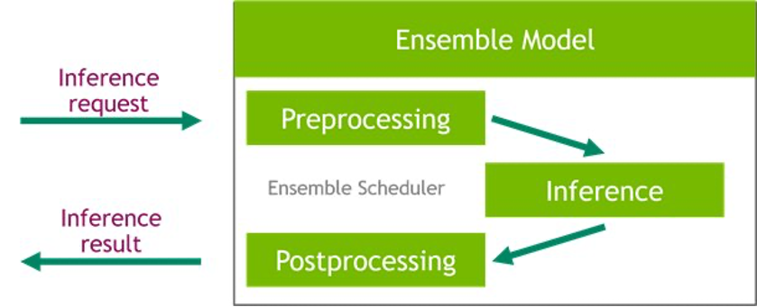
Triton Inference Server greatly simplifies the deployment of AI models at scale in production. Triton Inference Server comes with a convenient solution that simplifies building preprocessing and postprocessing pipelines. The Triton Inference Server platform provides the ensemble scheduler, which is responsible for pipelining models participating in the inference process while ensuring efficiency and optimizing throughput. Using ensemble models can avoid the overhead of transferring intermediate tensors and minimize the number of requests that must be sent to Triton.

In this notebook, we show how to use the ensemble feature for building a pipeline of data preprocessing with XGBoost model inference, and you can extrapolate from it to add custom postprocessing to the pipeline.

Set up the environment

We begin by setting up the required environment. We install the dependencies required to package our model pipeline and run inferences using Triton Inference Server. We also define the AWS Identity and Access Management (IAM) role that will give SageMaker access to the model artifacts and the NVIDIA Triton Amazon Elastic Container Registry (Amazon ECR) image. See the following code:

import boto3
import sagemaker
from sagemaker import get_execution_role
import pandas as pd
import numpy as np
import subprocess
sess = boto3.Session()
sm = sess.client("sagemaker")
##NOTE :Replace with your S3 bucket name
default_bucket="" 
sagemaker_session = sagemaker.Session(default_bucket=default_bucket)

##NOTE : Make sure to have SageMakerFullAccess permission to the below IAM Role
role = get_execution_role()
client = boto3.client("sagemaker-runtime")
s3_bucket = sagemaker_session.default_bucket()

##NOTE : Latest SageMaker DLCs can be found here, please change region and account ids accordingly - https://github.com/aws/deep-learning-containers/blob/master/available_images.md

triton_image_uri = (
"{account_id}.dkr.ecr.{region}.{base}/sagemaker-tritonserver:23.02-py3".format(
account_id=account_id_map[region], region=region, base=base
))

Create a Conda environment for preprocessing dependencies

The Python backend in Triton requires us to use a Conda environment for any additional dependencies. In this case, we use the Python backend to preprocess the raw data before feeding it into the XGBoost model that is running in the FIL backend. Even though we originally used RAPIDS cuDF and cuML to do the data preprocessing, here we use Pandas and scikit-learn as preprocessing dependencies during inference. We do this for three reasons:

• We show how to create a Conda environment for your dependencies and how to package it in the format expected by Triton’s Python backend.
• By showing the preprocessing model running in the Python backend on the CPU while the XGBoost runs on the GPU in the FIL backend, we illustrate how each model in Triton’s ensemble pipeline can run on a different framework backend as well as different hardware configurations.
• It highlights how the RAPIDS libraries (cuDF, cuML) are compatible with their CPU counterparts (Pandas, scikit-learn). For example, we can show how LabelEncoders created in cuML can be used in scikit-learn and vice versa.

We follow the instructions from the Triton documentation for packaging preprocessing dependencies (scikit-learn and Pandas) to be used in the Python backend as a Conda environment TAR file. The bash script create_prep_env.sh creates the Conda environment TAR file, then we move it into the preprocessing model directory. See the following code:

#!/bin/bash

conda create -y -n preprocessing_env python=3.8
source /opt/conda/etc/profile.d/conda.sh
conda activate preprocessing_env
export PYTHONNOUSERSITE=True
conda install -y -c conda-forge pandas scikit-learn
pip install conda-pack
conda-pack

After we run the preceding script, it generates preprocessing_env.tar.gz, which we copy to the preprocessing directory:

!cp preprocessing_env.tar.gz model_cpu_repository/preprocessing/
!cp preprocessing_env.tar.gz model_gpu_repository/preprocessinggpu/

Set up preprocessing with the Triton Python backend

For preprocessing, we use Triton’s Python backend to perform tabular data preprocessing (categorical encoding) during inference for raw data requests coming into the server. For more information about the preprocessing that was done during training, refer to the training notebook.

The Python backend enables preprocessing, postprocessing, and any other custom logic to be implemented in Python and served with Triton. Using Triton on SageMaker requires us to first set up a model repository folder containing the models we want to serve. We have already set up a model for Python data preprocessing called preprocessing in cpu_model_repository and gpu_model_repository.

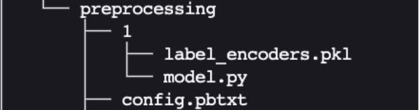
Triton has specific requirements for model repository layout. Within the top-level model repository directory, each model has its own subdirectory containing the information for the corresponding model. Each model directory in Triton must have at least one numeric subdirectory representing a version of the model. The value 1 represents version 1 of our Python preprocessing model. Each model is run by a specific backend, so within each version subdirectory there must be the model artifact required by that backend. For this example, we use the Python backend, which requires the Python file you’re serving to be called model.py, and the file needs to implement certain functions. If we were using a PyTorch backend, a model.pt file would be required, and so on. For more details on naming conventions for model files, refer to Model Files.

The model.py Python file we use here implements all the tabular data preprocessing logic to convert raw data into features that can be fed into our XGBoost model.

Every Triton model must also provide a config.pbtxt file describing the model configuration. To learn more about the config settings, refer to Model Configuration. Our config.pbtxt file specifies the backend as python and all the input columns for raw data along with preprocessed output, which consists of 15 features. We also specify we want to run this Python preprocessing model on the CPU. See the following code:

name: "preprocessing"
backend: "python"
max_batch_size: 882352
input [
    {
        name: "User"
        data_type: TYPE_FP32
        dims: [ 1 ]
    },
    {
        name: "Card"
        data_type: TYPE_FP32
        dims: [ 1 ]
    },
    {
        name: "Year"
        data_type: TYPE_FP32
        dims: [ 1 ]
    },
    {
        name: "Month"
        data_type: TYPE_FP32
        dims: [ 1 ]
    },
    {
        name: "Day"
        data_type: TYPE_FP32
        dims: [ 1 ]
    },
    {
        name: "Time"
        data_type: TYPE_STRING
        dims: [ 1 ]
    },
    {
        name: "Amount"
        data_type: TYPE_STRING
        dims: [ 1 ]
    },
    {
        name: "Use Chip"
        data_type: TYPE_STRING
        dims: [ 1 ]
    },
    {
        name: "Merchant Name"
        data_type: TYPE_STRING
        dims: [ 1 ]
    },
    {
        name: "Merchant City"
        data_type: TYPE_STRING
        dims: [ 1 ]
    },
    {
        name: "Merchant State"
        data_type: TYPE_STRING
        dims: [ 1 ]
    },
    {
        name: "Zip"
        data_type: TYPE_STRING
        dims: [ 1 ]
    },
    {
        name: "MCC"
        data_type: TYPE_STRING
        dims: [ 1 ]
    },
    {
        name: "Errors?"
        data_type: TYPE_STRING
        dims: [ 1 ]
    }
    
]
output [
    {
        name: "OUTPUT"
        data_type: TYPE_FP32
        dims: [ 15 ]
    }
]

instance_group [
    {
        count: 1
        kind: KIND_CPU
    }
]
parameters: {
  key: "EXECUTION_ENV_PATH",
  value: {string_value: "$$TRITON_MODEL_DIRECTORY/preprocessing_env.tar.gz"}
}

Set up a tree-based ML model for the FIL backend

Next, we set up the model directory for a tree-based ML model like XGBoost, which will be using the FIL backend.

The expected layout for cpu_memory_repository and gpu_memory_repository are similar to the one we showed earlier.

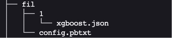
Here, FIL is the name of the model. We can give it a different name like xgboost if we want to. 1 is the version subdirectory, which contains the model artifact. In this case, it’s the xgboost.json model that we saved. Let’s create this expected layout:

# move saved xgboost model into fil model directory
!mkdir -p model_cpu_repository/fil/1
!cp xgboost.json model_cpu_repository/fil/1/
!cp xgboost.json model_gpu_repository/filgpu/1/

We need to have the configuration file config.pbtxt describing the model configuration for the tree-based ML model, so that the FIL backend in Triton can understand how to serve it. For more information, refer to the latest generic Triton configuration options and the configuration options specific to the FIL backend. We focus on just a few of the most common and relevant options in this example.

Create config.pbtxt for model_cpu_repository:

USE_GPU =False
FIL_MODEL_DIR = "./model_cpu_repository/fil"

# Maximum size in bytes for input and output arrays. If you are
# using Triton 21.11 or higher, all memory allocations will make
# use of Triton's memory pool, which has a default size of
# 67_108_864 bytes
MAX_MEMORY_BYTES = 60_000_000
NUM_FEATURES = 15
NUM_CLASSES = 2
bytes_per_sample = (NUM_FEATURES + NUM_CLASSES) * 4
max_batch_size = MAX_MEMORY_BYTES // bytes_per_sample

IS_CLASSIFIER = True
model_format = "xgboost_json"

# Select deployment hardware (GPU or CPU)
if USE_GPU:
    instance_kind = "KIND_GPU"
else:
    instance_kind = "KIND_CPU"

# whether the model is doing classification or regression
if IS_CLASSIFIER:
    classifier_string = "true"
else:
    classifier_string = "false"

# whether to predict probabilites or not
predict_proba = False

if predict_proba:
    predict_proba_string = "true"
else:
    predict_proba_string = "false"

config_text = f"""backend: "fil"
max_batch_size: {max_batch_size}
input [                                 
 {{  
    name: "input__0"
    data_type: TYPE_FP32
    dims: [ {NUM_FEATURES} ]                    
  }} 
]
output [
 {{
    name: "output__0"
    data_type: TYPE_FP32
    dims: [ 1 ]
  }}
]
instance_group [{{ kind: {instance_kind} }}]
parameters [
  {{
    key: "model_type"
    value: {{ string_value: "{model_format}" }}
  }},
  {{
    key: "predict_proba"
    value: {{ string_value: "{predict_proba_string}" }}
  }},
  {{
    key: "output_class"
    value: {{ string_value: "{classifier_string}" }}
  }},
  {{
    key: "threshold"
    value: {{ string_value: "0.5" }}
  }},
  {{
    key: "storage_type"
    value: {{ string_value: "AUTO" }}
  }}
]

dynamic_batching {{}}"""

config_path = os.path.join(FIL_MODEL_DIR, "config.pbtxt")
with open(config_path, "w") as file_:
    file_.write(config_text)

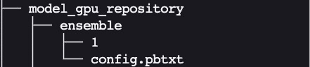
Similarly, set up config.pbtxt for model_gpu_repository (note the difference is USE_GPU = True):

USE_GPU = True
FIL_MODEL_DIR = "./model_gpu_repository/filgpu"

# Maximum size in bytes for input and output arrays. If you are
# using Triton 21.11 or higher, all memory allocations will make
# use of Triton's memory pool, which has a default size of
# 67_108_864 bytes
MAX_MEMORY_BYTES = 60_000_000
NUM_FEATURES = 15
NUM_CLASSES = 2
bytes_per_sample = (NUM_FEATURES + NUM_CLASSES) * 4
max_batch_size = MAX_MEMORY_BYTES // bytes_per_sample

IS_CLASSIFIER = True
model_format = "xgboost_json"

# Select deployment hardware (GPU or CPU)
if USE_GPU:
    instance_kind = "KIND_GPU"
else:
    instance_kind = "KIND_CPU"

# whether the model is doing classification or regression
if IS_CLASSIFIER:
    classifier_string = "true"
else:
    classifier_string = "false"

# whether to predict probabilites or not
predict_proba = False

if predict_proba:
    predict_proba_string = "true"
else:
    predict_proba_string = "false"

config_text = f"""backend: "fil"
max_batch_size: {max_batch_size}
input [                                 
 {{  
    name: "input__0"
    data_type: TYPE_FP32
    dims: [ {NUM_FEATURES} ]                    
  }} 
]
output [
 {{
    name: "output__0"
    data_type: TYPE_FP32
    dims: [ 1 ]
  }}
]
instance_group [{{ kind: {instance_kind} }}]
parameters [
  {{
    key: "model_type"
    value: {{ string_value: "{model_format}" }}
  }},
  {{
    key: "predict_proba"
    value: {{ string_value: "{predict_proba_string}" }}
  }},
  {{
    key: "output_class"
    value: {{ string_value: "{classifier_string}" }}
  }},
  {{
    key: "threshold"
    value: {{ string_value: "0.5" }}
  }},
  {{
    key: "storage_type"
    value: {{ string_value: "AUTO" }}
  }}
]

dynamic_batching {{}}"""

config_path = os.path.join(FIL_MODEL_DIR, "config.pbtxt")
with open(config_path, "w") as file_:
    file_.write(config_text)

Set up an inference pipeline of the data preprocessing Python backend and FIL backend using ensembles

Now we’re ready to set up the inference pipeline for data preprocessing and tree-based model inference using an ensemble model. An ensemble model represents a pipeline of one or more models and the connection of input and output tensors between those models. Here we use the ensemble model to build a pipeline of data preprocessing in the Python backend followed by XGBoost in the FIL backend.

The expected layout for the ensemble model directory is similar to the ones we showed previously:

# create model version directory for ensemble CPU model
!mkdir -p model_cpu_repository/ensemble/1
# create model version directory for ensemble GPU model
!mkdir -p model_gpu_repository/ensemble/1

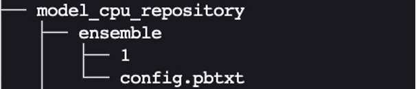
We created the ensemble model’s config.pbtxt following the guidance in Ensemble Models. Importantly, we need to set up the ensemble scheduler in config.pbtxt, which specifies the data flow between models within the ensemble. The ensemble scheduler collects the output tensors in each step, and provides them as input tensors for other steps according to the specification.

Package the model repository and upload to Amazon S3

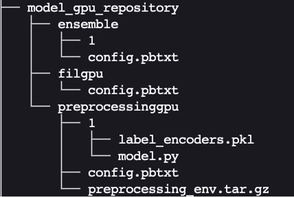
Finally, we end up with the following model repository directory structure, containing a Python preprocessing model and its dependencies along with the XGBoost FIL model and the model ensemble.

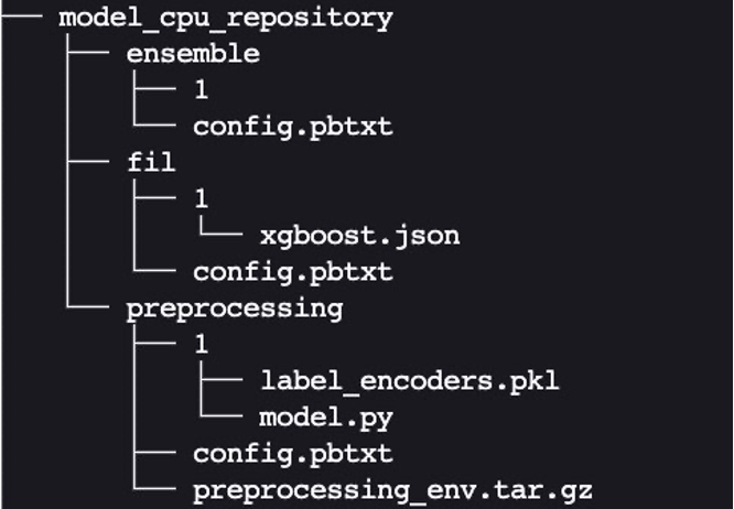
We package the directory and its contents as model.tar.gz for uploading to Amazon Simple Storage Service (Amazon S3). We have two options in this example: using a CPU-based instance or a GPU-based instance. A GPU-based instance is more suitable when you need higher processing power and want to use CUDA cores.

Create and upload the model package for a CPU-based instance (optimized for CPU) with the following code:

!tar —exclude='.ipynb_checkpoints' -czvf model-cpu.tar.gz -C model_cpu_repository .

model_uri_cpu = sagemaker_session.upload_data(
path="model-cpu.tar.gz", key_prefix="triton-fil-mme-ensemble"
)

Create and upload the model package for a GPU-based instance (optimized for GPU) with the following code:

!tar —exclude='.ipynb_checkpoints' -czvf model-gpu.tar.gz -C model_gpu_repository .

model_uri_cpu = sagemaker_session.upload_data(
path="model-gpu.tar.gz", key_prefix="triton-fil-mme-ensemble"
)

Create a SageMaker endpoint

We now have the model artifacts stored in an S3 bucket. In this step, we can also provide the additional environment variable SAGEMAKER_TRITON_DEFAULT_MODEL_NAME, which specifies the name of the model to be loaded by Triton. The value of this key should match the folder name in the model package uploaded to Amazon S3. This variable is optional in the case of a single model. In the case of ensemble models, this key has to be specified for Triton to start up in SageMaker.

Additionally, you can set SAGEMAKER_TRITON_BUFFER_MANAGER_THREAD_COUNT and SAGEMAKER_TRITON_THREAD_COUNT for optimizing the thread counts.

# Set the primary path for where all the models are stored on S3 bucket
model_location = f"s3://{s3_bucket}/triton-fil-mme-ensemble/"
sm_model_name = f"{user_profile}" + time.strftime("%Y-%m-%d-%H-%M-%S", time.gmtime())

container = {
 "Image": triton_image_uri,
 "ModelDataUrl": model_location,
"Mode": "MultiModel",
 "Environment": {
 "SAGEMAKER_TRITON_DEFAULT_MODEL_NAME": "ensemble",
# "SAGEMAKER_TRITON_DEFAULT_MODEL_NAME": model_uri.rsplit('/')[-2], #m_name,
# "SAGEMAKER_TRITON_LOG_VERBOSE": "true", #"200",
# "SAGEMAKER_TRITON_SHM_DEFAULT_BYTE_SIZE" : "20000000", #"1677721600", #"16777216000", "16777216"
# "SAGEMAKER_TRITON_SHM_GROWTH_BYTE_SIZE": "1048576"
},
}

create_model_response = sm.create_model(
 ModelName=sm_model_name, ExecutionRoleArn=role, PrimaryContainer=container
)

We use the preceding model to create an endpoint configuration where we can specify the type and number of instances we want in the endpoint

eendpoint_config_name = f"{user_profile}" + time.strftime("%Y-%m-%d-%H-%M-%S", time.gmtime())

create_endpoint_config_response = sm.create_endpoint_config(
 EndpointConfigName=endpoint_config_name,
 ProductionVariants=[
 {
 "InstanceType": "ml.g4dn.xlarge",
 "InitialVariantWeight": 1,
 "InitialInstanceCount": 1,
 "ModelName": sm_model_name,
 "VariantName": "AllTraffic",
 }
 ],
)

We use this endpoint configuration to create a SageMaker endpoint and wait for the deployment to finish. With SageMaker MMEs, we have the option to host multiple ensemble models by repeating this process, but we stick with one deployment for this example:

endpoint_name = f"{studio_user_profile_output}-lab1-" + time.strftime("%Y-%m-%d-%H-%M-%S", time.gmtime())
create_endpoint_response = sm.create_endpoint(
 EndpointName=endpoint_name, EndpointConfigName=endpoint_config_name
)

The status will change to InService when the deployment is successful.

Invoke your model hosted on the SageMaker endpoint

After the endpoint is running, we can use some sample raw data to perform inference using JSON as the payload format. For the inference request format, Triton uses the KFServing community standard inference protocols. See the following code:

data_infer = pd.read_csv("data_infer.csv")
STR_COLUMNS = [
    "Time",
    "Amount",
    "Zip",
    "MCC",
    "Merchant Name",
    "Use Chip",
    "Merchant City",
    "Merchant State",
    "Errors?",
]

batch_size = len(data_infer)

payload = {}
payload["inputs"] = []
data_dict = {}
for col_name in data_infer.columns:
    data_dict[col_name] = {}
    data_dict[col_name]["name"] = col_name
    if col_name in STR_COLUMNS:
        data_dict[col_name]["data"] = data_infer[col_name].astype(str).tolist()
        data_dict[col_name]["datatype"] = "BYTES"
    else:
        data_dict[col_name]["data"] = data_infer[col_name].astype("float32").tolist()
        data_dict[col_name]["datatype"] = "FP32"
    data_dict[col_name]["shape"] = [batch_size, 1]
    payload["inputs"].append(data_dict[col_name])
#Invoke the endpoint
# Change the TargetModel to either CPU or GPU
response = client.invoke_endpoint(
 EndpointName=endpoint_name, ContentType="application/octet-stream", Body=json.dumps(payload),TargetModel="model-cpu.tar.gz",
)

#Read the results
response_body = json.loads(response["Body"].read().decode("utf8"))
predictions = response_body["outputs"][0]["data"]

CLASS_LABELS = ["NOT FRAUD", "FRAUD"]
predictions = [CLASS_LABELS[int(idx)] for idx in predictions]
print(predictions)

The notebook referred in the blog can be found in the GitHub repository.

Best practices

In addition to the options to fine-tune the settings of the FIL backend we mentioned earlier, data scientists can also ensure that the input data for the backend is optimized for processing by the engine. Whenever possible, input data in row-major format into the GPU array. Other formats will require internal conversion and take up cycles, decreasing performance.

Due to the way FIL data structures are maintained in GPU memory, be mindful of the tree depth. The deeper the tree depth, the larger your GPU memory footprint will be.

Use the instance_group_count parameter to add worker processes and increase the throughput of the FIL backend, which will result in larger CPU and GPU memory consumption. In addition, consider SageMaker-specific variables that are available to increase the throughput, such as HTTP threads, HTTP buffer size, batch size, and max delay.

Conclusion

In this post, we dove deep into the FIL backend that Triton Inference Server supports on SageMaker. This backend provides for both CPU and GPU acceleration of your tree-based models such as the popular XGBoost algorithm. There are many options to consider to get the best performance for inference, such as batch sizes, data input formats, and other factors that can be tuned to meet your needs. SageMaker allows you to use this capability with single and multi-model endpoints to balance of performance and cost savings.

We encourage you to take the information in this post and see if SageMaker can meet your hosting needs to serve tree-based models, meeting your requirements for cost reduction and workload performance.

The notebook referenced in this post can be found in the SageMaker examples GitHub repository. Furthermore, you can find the latest documentation on the FIL backend on GitHub.

About the Authors

Raghu Ramesha is an Senior ML Solutions Architect with the Amazon SageMaker Service team. He focuses on helping customers build, deploy, and migrate ML production workloads to SageMaker at scale. He specializes in machine learning, AI, and computer vision domains, and holds a master’s degree in Computer Science from UT Dallas. In his free time, he enjoys traveling and photography.

James Park is a Solutions Architect at Amazon Web Services. He works with Amazon.com to design, build, and deploy technology solutions on AWS, and has a particular interest in AI and machine learning. In his spare time he enjoys seeking out new cultures, new experiences,  and staying up to date with the latest technology trends.

Dhawal Patel is a Principal Machine Learning Architect at AWS. He has worked with organizations ranging from large enterprises to mid-sized startups on problems related to distributed computing and artificial intelligence. He focuses on deep learning, including NLP and computer vision domains. He helps customers achieve high-performance model inference on Amazon SageMaker.

Jiahong Liu is a Solution Architect on the Cloud Service Provider team at NVIDIA. He assists clients in adopting machine learning and AI solutions that leverage NVIDIA accelerated computing to address their training and inference challenges. In his leisure time, he enjoys origami, DIY projects, and playing basketball.

Kshitiz Gupta is a Solutions Architect at NVIDIA. He enjoys educating cloud customers about the GPU AI technologies NVIDIA has to offer and assisting them with accelerating their machine learning and deep learning applications. Outside of work, he enjoys running, hiking and wildlife watching.