This post is co-written with Jonathan Jung, Mike Band, Michael Chi, and Thompson Bliss at the National Football League.
A coverage scheme refers to the rules and responsibilities of each football defender tasked with stopping an offensive pass. It is at the core of understanding and analyzing any football defensive strategy. Classifying the coverage scheme for every pass play will provide insights of the football game to teams, broadcasters, and fans alike. For instance, it can reveal the preferences of play callers, allow deeper understanding of how respective coaches and teams continuously adjust their strategies based on their opponent’s strengths, and enable the development of new defensive-oriented analytics such as uniqueness of coverages (Seth et al.). However, manual identification of these coverages on a per-play basis is both laborious and difficult because it requires football specialists to carefully inspect the game footage. There is a need for an automated coverage classification model that can scale effectively and efficiently to reduce cost and turnaround time.
The NFL’s Next Gen Stats captures real-time location, speed, and more for every player and play of NFL football games, and derives various advanced stats covering different aspects of the game. Through a collaboration between the Next Gen Stats team and the Amazon ML Solutions Lab, we have developed the machine learning (ML)-powered stat of coverage classification that accurately identifies the defense coverage scheme based on the player tracking data. The coverage classification model is trained using Amazon SageMaker, and the stat has been launched for the 2022 NFL season.
In this post, we deep dive into the technical details of this ML model. We describe how we designed an accurate, explainable ML model to make coverage classification from player tracking data, followed by our quantitative evaluation and model explanation results.
Problem formulation and challenges
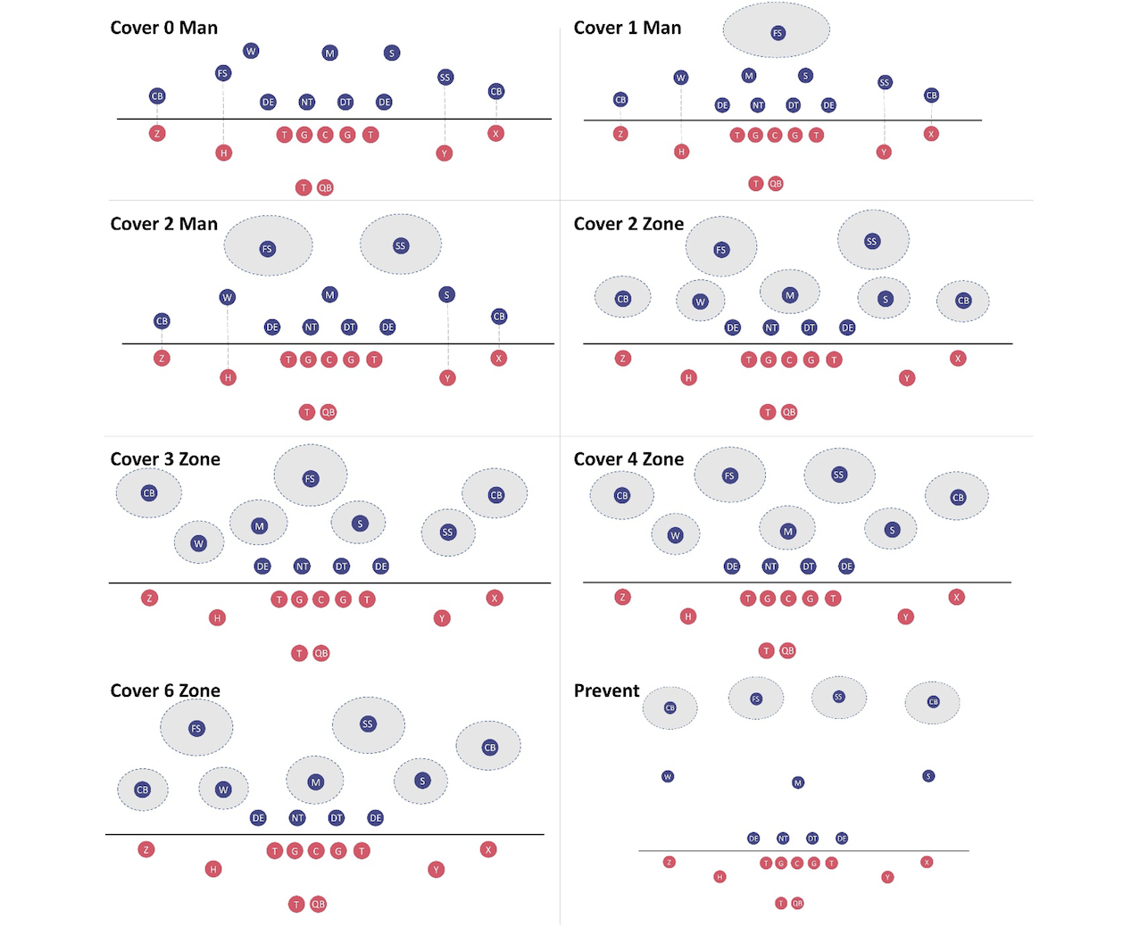
We define the defensive coverage classification as a multi-class classification task, with three types of man coverage (where each defensive player covers a certain offensive player) and five types of zone coverage (each defensive player covers a certain area on the field). These eight classes are visually depicted in the following figure: Cover 0 Man, Cover 1 Man, Cover 2 Man, Cover 2 Zone, Cover 3 Zone, Cover 4 Zone, Cover 6 Zone, and Prevent (also zone coverage). Circles in blue are the defensive players laid out in a particular type of coverage; circles in red are the offensive players. A full list of the player acronyms is provided in the appendix at the end of this post.

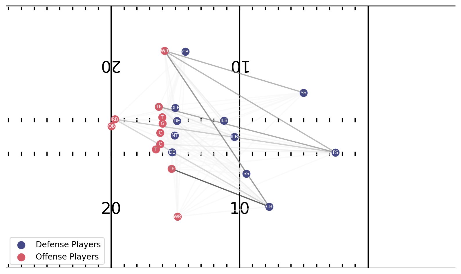
The following visualization shows an example play, with the location of all offensive and defensive players at the start of the play (left) and in the middle of the same play (right). To make the correct coverage identification, a multitude of information over time must be accounted for, including the way defenders lined up before the snap and the adjustments to offensive player movement once the ball is snapped. This poses the challenge for the model to capture spatial-temporal, and often subtle movement and interaction among the players.

Another key challenge faced by our partnership is the inherent ambiguity around the deployed coverage schemes. Beyond the eight commonly known coverage schemes, we identified adjustments in more specific coverage calls that lead to ambiguity among the eight general classes for both manual charting and model classification. We tackle these challenges using improved training strategies and model explanation. We describe our approaches in detail in the following section.
Explainable coverage classification framework
We illustrate our overall framework in the following figure, with the input of player tracking data and coverage labels starting at the top of the figure.

Feature engineering
Game tracking data is captured at 10 frames per second, including the player location, speed, acceleration, and orientation. Our feature engineering constructs sequences of play features as the input for model digestion. For a given frame, our features are inspired by the 2020 Big Data Bowl Kaggle Zoo solution (Gordeev et al.): we construct an image for each time step with the defensive players at the rows and offensive players at the columns. The pixel of the image therefore represents the features for the intersecting pair of players. Different from Gordeev et al., we extract a sequence of the frame representations, which effectively generates a mini-video to characterize the play.
The following figure visualizes how the features evolve over time in correspondence to two snapshots of an example play. For visual clarity, we only show four features out of all the ones we extracted. “LOS” in the figure stands for the line of scrimmage, and the x-axis refers to the horizontal direction to the right of the football field. Notice how the feature values, indicated by the colorbar, evolve over time in correspondence to the player movement. Altogether, we construct two sets of features as follows:
- Defender features consisting of the defender position, speed, acceleration, and orientation, on the x-axis (horizontal direction to the right of the football field) and y-axis (vertical direction to the top of the football field)
- Defender-offense relative features consisting of the same attributes, but calculated as the difference between the defensive and offensive players

CNN module
We utilize a convolutional neural network (CNN) to model the complex player interactions similar to the Open Source Football (Baldwin et al.) and Big Data Bowl Kaggle Zoo solution (Gordeev et al.). The image obtained from feature engineering facilitated the modeling of each play frame through a CNN. We modified the convolutional (Conv) block utilized by the Zoo solution (Gordeev et al.) with a branching structure that is comprised of a shallow one-layer CNN and a deep three-layer CNN. The convolution layer utilizes a 1×1 kernel internally: having the kernel look at each player pair individually ensures that the model is invariant to the player ordering. For simplicity, we order the players based on their NFL ID for all play samples. We obtain the frame embeddings as the output of the CNN module.
Temporal modeling
Within the short play period lasting just a few seconds, it contains rich temporal dynamics as key indicators to identify the coverage. The frame-based CNN modeling, as used in the Zoo solution (Gordeev et al.), has not accounted for the temporal progression. To tackle this challenge, we design a self-attention module (Vaswani et al.), stacked on top of the CNN, for temporal modeling. During training, it learns to aggregate the individual frames by weighing them differently (Alammar et al.). We will compare it with a more conventional, bidirectional LSTM approach in the quantitative evaluation. The learned attention embeddings as the output are then averaged to obtain the embedding of the whole play. Finally, a fully connected layer is connected to determine the coverage class of the play.
Model ensemble and label smoothing
Ambiguity among the eight coverage schemes and their imbalanced distribution make the clear separation among coverages challenging. We utilize the model ensemble to tackle these challenges during model training. Our study finds that a voting-based ensemble, one of the most simplistic ensemble methods, actually outperforms more complex approaches. In this method, each base model has the same CNN-attention architecture and is trained independently from different random seeds. The final classification takes the average over the outputs from all base models.
We further incorporate label smoothing (Müller et al.) into the cross-entropy loss to handle the potential noise in manual charting labels. Label smoothing steers the annotated coverage class slightly towards the remaining classes. The idea is to encourage the model to adapt to the inherent coverage ambiguity instead of overfitting to any biased annotations.
Quantitative evaluation
We utilize 2018–2020 season data for model training and validation, and 2021 season data for model evaluation. Each season consists of around 17,000 plays. We perform a five-fold cross-validation to select the best model during training, and perform hyperparameter optimization to select the best settings on multiple model architecture and training parameters.
To evaluate the model performance, we compute the coverage accuracy, F1 score, top-2 accuracy, and accuracy of the easier man vs. zone task. The CNN-based Zoo model used in Baldwin et al. is the most relevant for coverage classification and we use it as the baseline. In addition, we consider improved versions of the baseline that incorporate the temporal modeling components for comparative study: a CNN-LSTM model that utilizes a bi-directional LSTM to perform the temporal modeling, and a single CNN-attention model without the ensemble and label smoothing components. The results are shown in the following table.
| Model | Test Accuracy 8 Coverages (%) | Top-2 Accuracy 8 Coverages (%) | F1 Score 8 Coverages | Test Accuracy Man vs. Zone (%) |
| Baseline: Zoo model | 68.8±0.4 | 87.7±0.1 | 65.8±0.4 | 88.4±0.4 |
| CNN-LSTM | 86.5±0.1 | 93.9±0.1 | 84.9±0.2 | 94.6±0.2 |
| CNN-attention | 87.7±0.2 | 94.7±0.2 | 85.9±0.2 | 94.6±0.2 |
| Ours: Ensemble of 5 CNN-attention models | 88.9±0.1 | 97.6±0.1 | 87.4±0.2 | 95.4±0.1 |
We observe that incorporation of the temporal modeling module significantly improves the baseline Zoo model that was based on a single frame. Compared to the strong baseline of the CNN-LSTM model, our proposed modeling components including the self-attention module, model ensemble, and labeling smoothing combined provide significant performance improvement. The final model is performant as demonstrated by the evaluation measures. In addition, we identify very high top-2 accuracy and a significant gap to the top-1 accuracy. This can be attributed to the coverage ambiguity: when the top classification is incorrect, the 2nd guess often matches human annotation.
Model explanations and results
To shed light on the coverage ambiguity and understand what the model utilized to arrive at a given conclusion, we perform analysis using model explanations. It consists of two parts: global explanations that analyze all learned embeddings jointly, and local explanations that zoom into individual plays to analyze the most important signals captured by the model.
Global explanations
In this stage, we analyze the learned play embeddings from the coverage classification model globally to discover any patterns that require manual review. We utilize t-distributed stochastic neighbor embedding (t-SNE) (Maaten et al.) that projects the play embeddings into 2D space such as a pair of similar embeddings have high probability on their distribution. We experiment with the internal parameters to extract stable 2D projections. The embeddings from stratified samples of 9,000 plays are visualized in following figure (left), with each dot representing a certain play. We find that the majority of each coverage scheme are well separated, demonstrating the classification capability gained by the model. We observe two important patterns and investigate them further.
Some plays are mixed into other coverage types, as shown in the following figure (right). These plays could potentially be mislabeled and deserve manual inspection. We design a K-Nearest Neighbors (KNN) classifier to automatically identify these plays and send them for expert review. The results show that most of them were indeed labeled incorrectly.

Next, we observe several overlapping regions among the coverage types, manifesting coverage ambiguity in certain scenarios. As an example, in the following figure, we separate Cover 3 Zone (green cluster on the left) and Cover 1 Man (blue cluster in the middle). These are two different single-high coverage concepts, where the main distinction is man vs. zone coverage. We design an algorithm that automatically identifies the ambiguity between these two classes as the overlapping region of the clusters. The result is visualized as the red dots in the following right figure, with 10 randomly sampled plays marked with a black “x” for manual review. Our analysis reveals that most of the play examples in this region involve some sort of pattern matching. In these plays, the coverage responsibilities are contingent upon how the offensive receivers’ routes are distributed, and adjustments can make the play look like a mix of zone and man coverages. One such adjustment we identified applies to Cover 3 Zone, when the cornerback (CB) to one side is locked into man coverage (“Man Everywhere he Goes” or MEG) and the other has a traditional zone drop.

Instance explanations
In the second stage, instance explanations zoom into the individual play of interest, and extract frame-by-frame player interaction highlights that contribute the most to the identified coverage scheme. This is achieved through the Guided GradCAM algorithm (Ramprasaath et al.). We utilize the instance explanations on low-confidence model predictions.
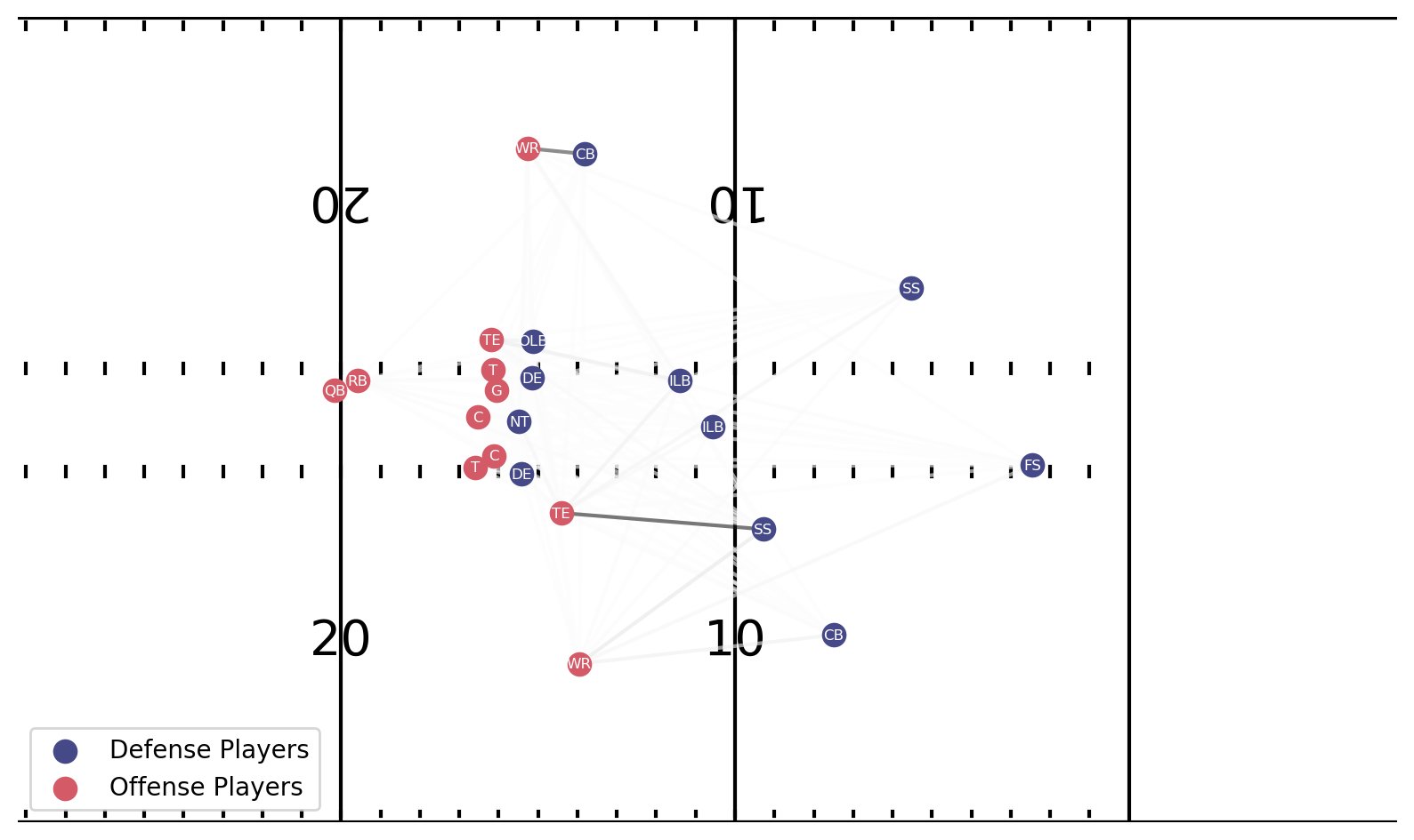
For the play we illustrated in the beginning of the post, the model predicted Cover 3 Zone with 44.5% probability and Cover 1 Man with 31.3% probability. We generate the explanation results for both classes as shown in the following figure. The line thickness annotates the interaction strength that contributes to the model’s identification.
The top plot for Cover 3 Zone explanation comes right after the ball snap. The CB on the offense’s right has the strongest interaction lines, because he is facing the QB and stays in place. He ends up squaring off and matching with the receiver on his side, who threatens him deep.
The bottom plot for Cover 1 Man explanation comes a moment later, as the play action fake is happening. One of the strongest interactions is with the CB to the offense’s left, who is dropping with the WR. Play footage reveals that he keeps his eyes on the QB before flipping around and running with the WR who is threatening him deep. The SS on the offense’s right also has a strong interaction with the TE on his side, as he starts to shuffle as the TE breaks inside. He ends up following him across the formation, but the TE starts to block him, indicating the play was likely a run-pass option. This explains the uncertainty of the model’s classification: the TE is sticking with the SS by design, creating biases in the data.
Conclusion
The Amazon ML Solutions Lab and NFL’s Next Gen Stats team jointly developed the defense coverage classification stat that was recently launched for the 2022 NFL football season. This post presented the ML technical details of this stat, including the modeling of the fast temporal progression, training strategies to handle the coverage class ambiguity, and comprehensive model explanations to speed up expert review on both global and instance levels.
The solution makes live defensive coverage tendencies and splits available to broadcasters in-game for the first time ever. Likewise, the model enables the NFL to improve its analysis of post-game results and better identify key matchups leading up to games.
If you’d like help accelerating your use of ML, please contact the Amazon ML Solutions Lab program.
Appendix
| Player position acronyms | |
| Defensive positions | |
| W | “Will” Linebacker, or the weak side LB |
| M | “Mike” Linebacker, or the middle LB |
| S | “Sam” Linebacker, or the strong side LB |
| CB | Cornerback |
| DE | Defensive End |
| DT | Defensive Tackle |
| NT | Nose Tackle |
| FS | Free Safety |
| SS | Strong Safety |
| S | Safety |
| LB | Linebacker |
| ILB | Inside Linebacker |
| OLB | Outside Linebacker |
| MLB | Middle Linebacker |
| Offensive positions | |
| X | Usually the number 1 wide receiver in an offense, they align on the LOS. In trips formations, this receiver is often aligned isolated on the backside. |
| Y | Usually the starting tight end, this player will often align in-line and to the opposite side as the X. |
| Z | Usually more of a slot receiver, this player will often align off the line of scrimmage and on the same side of the field as the tight end. |
| H | Traditionally a fullback, this player is more often a third wide receiver or a second tight end in the modern league. They can align all over the formation, but are almost always off the line of scrimmage. Depending on the team, this player could also be designated as an F. |
| T | The featured running back. Other than empty formations, this player will align in the backfield and be a threat to receive the handoff. |
| QB | Quarterback |
| C | Center |
| G | Guard |
| RB | Running Back |
| FB | Fullback |
| WR | Wide Receiver |
| TE | Tight End |
| LG | Left Guard |
| RG | Right Guard |
| T | Tackle |
| LT | Left Tackle |
| RT | Right Tackle |
References
- Tej Seth, Ryan Weisman, “PFF Data Study: Coverage scheme uniqueness for each team and what that means for coaching changes”, https://www.pff.com/news/nfl-pff-data-study-coverage-scheme-uniqueness-for-each-team-and-what-that-means-for-coaching-changes
- Ben Baldwin. “Computer Vision with NFL Player Tracking Data using torch for R: Coverage classification Using CNNs.” https://www.opensourcefootball.com/posts/2021-05-31-computer-vision-in-r-using-torch/
- Dmitry Gordeev, Philipp Singer. “1st place solution The Zoo.” https://www.kaggle.com/c/nfl-big-data-bowl-2020/discussion/119400
- Vaswani, Ashish, Noam Shazeer, Niki Parmar, Jakob Uszkoreit, Llion Jones, Aidan N. Gomez, Łukasz Kaiser, and Illia Polosukhin. “Attention is all you need.” Advances in neural information processing systems 30 (2017).
- Jay Alammar. “The Illustrated Transformer.” https://jalammar.github.io/illustrated-transformer/
- Müller, Rafael, Simon Kornblith, and Geoffrey E. Hinton. “When does label smoothing help?.” Advances in neural information processing systems 32 (2019).
- Van der Maaten, Laurens, and Geoffrey Hinton. “Visualizing data using t-SNE.” Journal of machine learning research 9, no. 11 (2008).
- Selvaraju, Ramprasaath R., Michael Cogswell, Abhishek Das, Ramakrishna Vedantam, Devi Parikh, and Dhruv Batra. “Grad-cam: Visual explanations from deep networks via gradient-based localization.” In Proceedings of the IEEE international conference on computer vision, pp. 618-626. 2017.
About the Authors
 Huan Song is an applied scientist at Amazon Machine Learning Solutions Lab, where he works on delivering custom ML solutions for high-impact customer use cases from a variety of industry verticals. His research interests are graph neural networks, computer vision, time series analysis and their industrial applications.
 Mohamad Al Jazaery is an applied scientist at Amazon Machine Learning Solutions Lab. He helps AWS customers identify and build ML solutions to address their business challenges in areas such as logistics, personalization and recommendations, computer vision, fraud prevention, forecasting and supply chain optimization. Prior to AWS, he obtained his MCS from West Virginia University and worked as computer vision researcher at Midea. Outside of work, he enjoys soccer and video games.
 Haibo Ding is a senior applied scientist at Amazon Machine Learning Solutions Lab. He is broadly interested in Deep Learning and Natural Language Processing. His research focuses on developing new explainable machine learning models, with the goal of making them more efficient and trustworthy for real-world problems. He obtained his Ph.D. from University of Utah and worked as a senior research scientist at Bosch Research North America before joining Amazon. Apart from work, he enjoys hiking, running, and spending time with his family.
 Lin Lee Cheong is an applied science manager with the Amazon ML Solutions Lab team at AWS. She works with strategic AWS customers to explore and apply artificial intelligence and machine learning to discover new insights and solve complex problems. She received her Ph.D. from Massachusetts Institute of Technology. Outside of work, she enjoys reading and hiking.
 Jonathan Jung is a Senior Software Engineer at the National Football League. He has been with the Next Gen Stats team for the last seven years helping to build out the platform from streaming the raw data, building out microservices to process the data, to building API’s that exposes the processed data. He has collaborated with the Amazon Machine Learning Solutions Lab in providing clean data for them to work with as well as providing domain knowledge about the data itself. Outside of work, he enjoys cycling in Los Angeles and hiking in the Sierras.
 Mike Band is a Senior Manager of Research and Analytics for Next Gen Stats at the National Football League. Since joining the team in 2018, he has been responsible for ideation, development, and communication of key stats and insights derived from player-tracking data for fans, NFL broadcast partners, and the 32 clubs alike. Mike brings a wealth of knowledge and experience to the team with a master’s degree in analytics from the University of Chicago, a bachelor’s degree in sport management from the University of Florida, and experience in both the scouting department of the Minnesota Vikings and the recruiting department of Florida Gator Football.
 Michael Chi is a Senior Director of Technology overseeing Next Gen Stats and Data Engineering at the National Football League. He has a degree in Mathematics and Computer Science from the University of Illinois at Urbana Champaign. Michael first joined the NFL in 2007 and has primarily focused on technology and platforms for football statistics. In his spare time, he enjoys spending time with his family outdoors.
 Thompson Bliss is a Manager, Football Operations, Data Scientist at the National Football League. He started at the NFL in February 2020 as a Data Scientist and was promoted to his current role in December 2021. He completed his master’s degree in Data Science at Columbia University in the City of New York in December 2019. He received a Bachelor of Science in Physics and Astronomy with minors in Mathematics and Computer Science at University of Wisconsin – Madison in 2018.