Amazon Lookout for Vision provides a machine learning (ML)-based anomaly detection service to identify normal images (i.e., images of objects without defects) vs anomalous images (i.e., images of objects with defects), types of anomalies (e.g., missing piece), and the location of these anomalies. Therefore, Lookout for Vision is popular among customers that look for automated solutions for industrial quality inspection (e.g., detecting abnormal products). However, customers’ datasets usually face two problems:
- The number of images with anomalies could be very low and might not reach anomalies/defect type minimum imposed by Lookout for Vision (~20).
- Normal images might not have enough diversity and might result in the model failing when environmental conditions such as lighting change in production
To overcome these problems, this post introduces an image augmentation pipeline that targets both problems: It provides a way to generate synthetic anomalous images by removing objects in images and generates additional normal images by introducing controlled augmentation such as gaussian noise, hue, saturation, pixel value scaling etc. We use the imgaug library to introduce augmentation to generate additional anomalous and normal images for the second problem. We use Amazon Sagemaker Ground Truth to generate object removal masks and the LaMa algorithm to remove objects for the first problem using image inpainting (object removal) techniques.
The rest of the post is organized as follows. In Section 3, we present the image augmentation pipeline for normal images. In Section 4, we present the image augmentation pipeline for abnormal images (aka synthetic defect generation). Section 5 illustrates the Lookout for Vision training results using the augmented dataset. Section 6 demonstrates how the Lookout for Vision model trained on synthetic data perform against real defects. In Section 7, we talk about cost estimation for this solution. All of the code we used for this post can be accessed here.
1. Solution overview
ML diagram
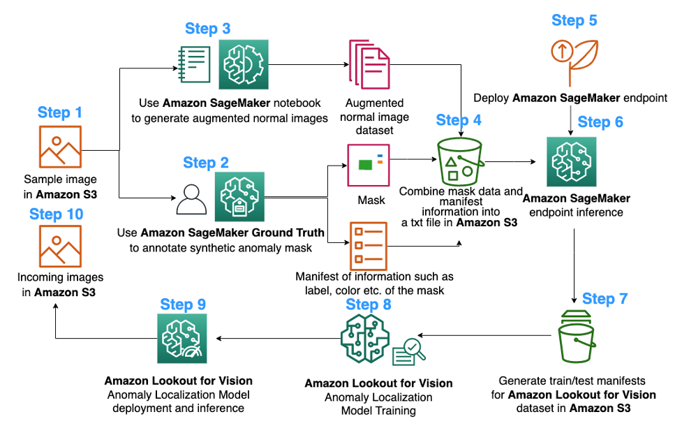
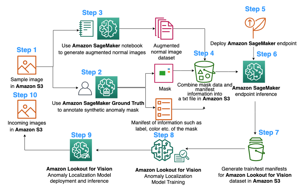
The following is the diagram of the proposed image augmentation pipeline for Lookout for Vision anomaly localization model training:

The diagram above starts by collecting a series of images (step 1). We augment the dataset by augmenting the normal images (step 3) and by using object removal algorithms (steps 2, 5-6). We then package the data in a format that can be consumed by Amazon Lookout for Vision (steps 7-8). Finally, in step 9, we use the packaged data to train a Lookout for Vision localization model.
This image augmentation pipeline gives customers flexibility to generate synthetic defects in the limited sample dataset, as well as add more quantity and variety to normal images. It would boost the performance of Lookout for Vision service, solving the lack of customer data issue and making the automated quality inspection process smoother.
2. Data preparation
From here to the end of the post, we use the public FICS-PCB: A Multi-Modal Image Dataset for Automated Printed Circuit Board Visual Inspection dataset licensed under a Creative Commons Attribution 4.0 International (CC BY 4.0) License to illustrate the image augmentation pipeline and the consequent Lookout for Vision training and testing. This dataset is designed to support the evaluation of automated PCB visual inspection systems. It was collected at the SeCurity and AssuraNce (SCAN) lab at the University of Florida. It can be accessed here.
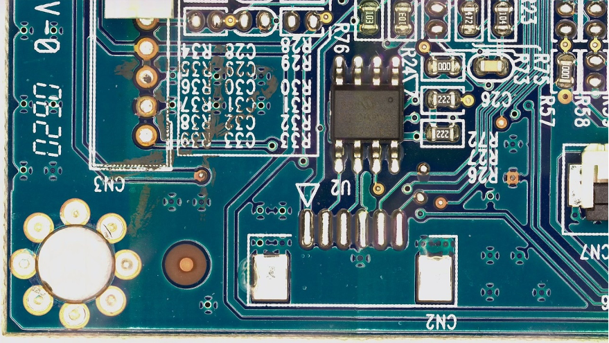
We start with the hypothesis that the customer only provides a single normal image of a PCB board (a s10 PCB sample) as the dataset. It can be seen as follows:

3. Image augmentation for normal images
The Lookout for Vision service requires at least 20 normal images and 20 anomalies per defect type. Since there is only one normal image from the sample data, we must generate more normal images using image augmentation techniques. From the ML standpoint, feeding multiple image transformations using different augmentation techniques can improve the accuracy and robustness of the model.
We’ll use imgaug for image augmentation of normal images. Imgaug is an open-source python package that lets you augment images in ML experiments.
First, we’ll install the imgaug library in an Amazon SageMaker notebook.
Next, we can install the python package named ‘IPyPlot’.
Then, we perform image augmentation of the original image using transformations including GammaContrast, SigmoidContrast, and LinearContrast, and adding Gaussian noise on the image.
import imageio
import imgaug as ia
import imgaug.augmenters as iaa
import ipyplot
input_img = imageio.imread('s10.png')
noise=iaa.AdditiveGaussianNoise(10,40)
input_noise=noise.augment_image(input_img)
contrast=iaa.GammaContrast((0.5, 2.0))
contrast_sig = iaa.SigmoidContrast(gain=(5, 10), cutoff=(0.4, 0.6))
contrast_lin = iaa.LinearContrast((0.6, 0.4))
input_contrast = contrast.augment_image(input_img)
sigmoid_contrast = contrast_sig.augment_image(input_img)
linear_contrast = contrast_lin.augment_image(input_img)
images_list=[input_img, input_contrast,sigmoid_contrast,linear_contrast,input_noise]
labels = ['Original', 'Gamma Contrast','SigmoidContrast','LinearContrast','Gaussian Noise Image']
ipyplot.plot_images(images_list,labels=labels,img_width=180)

Since we need at least 20 normal images, and the more the better, we generated 10 augmented images for each of the 4 transformations shown above as our normal image dataset. In the future, we plan to also transform the images to be positioned at difference locations and different angels so that the trained model can be less sensitive to the placement of the object relative to the fixed camera.
4. Synthetic defect generation for augmentation of abnormal images
In this section, we present a synthetic defect generation pipeline to augment the number of images with anomalies in the dataset. Note that, as opposed to the previous section where we create new normal samples from existing normal samples, here, we create new anomaly images from normal samples. This is an attractive feature for customers that completely lack this kind of images in their datasets, e.g., removing a component of the normal PCB board. This synthetic defect generation pipeline has three steps: first, we generate synthetic masks from source (normal) images using Amazon SageMaker Ground Truth. In this post, we target at a specific defect type: missing component. This mask generation provides a mask image and a manifest file. Second, the manifest file must be modified and converted to an input file for a SageMaker endpoint. And third, the input file is input to an Object Removal SageMaker endpoint responsible of removing the parts of the normal image indicated by the mask. This endpoint provides the resulting abnormal image.
4.1 Generate synthetic defect masks using Amazon SageMaker Ground Truth
Amazon Sagemaker Ground Truth for data labeling
Amazon SageMaker Ground Truth is a data labeling service that makes it easy to label data and gives you the option to use human annotators through Amazon Mechanical Turk, third-party vendors, or your own private workforce. You can follow this tutorial to set up a labeling job.
In this section, we’ll show how we use Amazon SageMaker Ground Truth to mark specific “components” in normal images to be removed in the next step. Note that a key contribution of this post is that we don’t use Amazon SageMaker Ground Truth in its traditional way (that is, to label training images). Here, we use it to generate a mask for future removal in normal images. These removals in normal images will generate the synthetic defects.
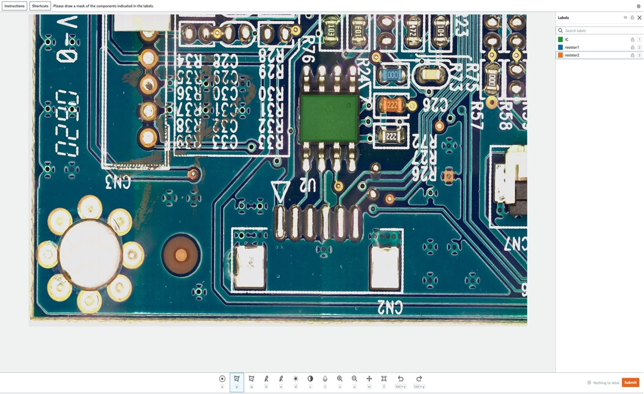
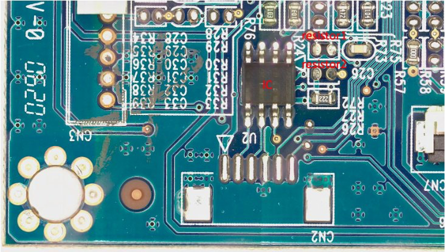
For the purpose of this post, in our labeling job we’ll artificially remove up to three components from the PCB board: IC, resistor1, and resistor2. After entering the labeling job as a labeler, you can select the label name and draw a mask of any shape around the component that you want to remove from the image as a synthetic defect. Note that you can’t include ‘_’ in the label name for this experiment, since we use ‘_’ to separate different metadata in the defect name later in the code.
In the following picture, we draw a green mask around IC (Integrated Circuit), a blue mask around resistor 1, and an orange mask around resistor 2.

After we select the submit button, Amazon SageMaker Ground Truth will generate an output mask with white background and a manifest file as follows:

{"source-ref":"s3://pcbtest22/label/s10.png","s10-label-ref":"s3://pcbtest22/label/s10-label/annotations/consolidated-annotation/output/0_2022-09-08T18:01:51.334016.png","s10-label-ref-metadata":{"internal-color-map":{"0":{"class-name":"BACKGROUND","hex-color":"#ffffff","confidence":0},"1":{"class-name":"IC","hex-color":"#2ca02c","confidence":0},"2":{"class-name":"resistor_1","hex-color":"#1f77b4","confidence":0},"3":{"class-name":"resistor_2","hex-color":"#ff7f0e","confidence":0}},"type":"groundtruth/semantic-segmentation","human-annotated":"yes","creation-date":"2022-09-08T18:01:51.498525","job-name":"labeling-job/s10-label"}}
Note that so far we haven’t generated any abnormal images. We just marked the three components that will be artificially removed and whose removal will generate abnormal images. Later, we’ll use both (1) the mask image above, and (2) the information from the manifest file as inputs for the abnormal image generation pipeline. The next section shows how to prepare the input for the SageMaker endpoint.
4.2 Prepare Input for SageMaker endpoint
Transform Amazon SageMaker Ground Truth manifest as a SageMaker endpoint input file
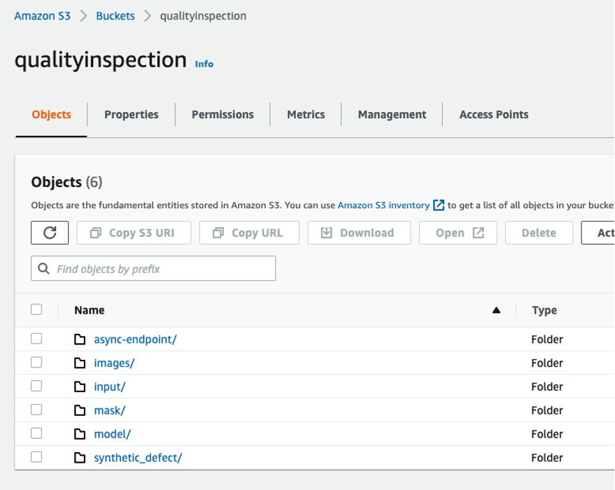
First, we set up an Amazon Simple Storage Service (Amazon S3) bucket to store all of the input and output for the image augmentation pipeline. In the post, we use an S3 bucket named qualityinspection. Then we generate all of the augmented normal images and upload them to this S3 bucket.
from PIL import Image
import os
import shutil
import boto3

s3=boto3.client('s3')

# make the image directory
dir_im="images"
if not os.path.isdir(dir_im):
    os.makedirs(dir_im)
# create augmented images from original image
input_img = imageio.imread('s10.png')

for i in range(10):
    noise=iaa.AdditiveGaussianNoise(scale=0.2*255)
    contrast=iaa.GammaContrast((0.5,2))
    contrast_sig = iaa.SigmoidContrast(gain=(5,20), cutoff=(0.25, 0.75))
    contrast_lin = iaa.LinearContrast((0.4,1.6))

    input_noise=noise.augment_image(input_img)
    input_contrast = contrast.augment_image(input_img)
    sigmoid_contrast = contrast_sig.augment_image(input_img)
    linear_contrast = contrast_lin.augment_image(input_img)

    im_noise = Image.fromarray(input_noise)
    im_noise.save(f'{dir_im}/input_noise_{i}.png')

    im_input_contrast = Image.fromarray(input_contrast)
    im_input_contrast.save(f'{dir_im}/contrast_sig_{i}.png')

    im_sigmoid_contrast = Image.fromarray(sigmoid_contrast)
    im_sigmoid_contrast.save(f'{dir_im}/sigmoid_contrast_{i}.png')

    im_linear_contrast = Image.fromarray(linear_contrast)
    im_linear_contrast.save(f'{dir_im}/linear_contrast_{i}.png')

# move original image to image augmentation folder
shutil.move('s10.png','images/s10.png')
# list all the images in the image directory
imlist =  [file for file in os.listdir(dir_im) if file.endswith('.png')]

# upload augmented images to an s3 bucket
s3_bucket='qualityinspection'
for i in range(len(imlist)):
    with open('images/'+imlist[i], 'rb') as data:
        s3.upload_fileobj(data, s3_bucket, 'images/'+imlist[i])

# get the image s3 locations
im_s3_list=[]
for i in range(len(imlist)):
    image_s3='s3://qualityinspection/images/'+imlist[i]
    im_s3_list.append(image_s3)
Next, we download the mask from Amazon SageMaker Ground Truth and upload it to a folder named ‘mask’ in that S3 bucket.
# download Ground Truth annotation mask image to local from the Ground Truth s3 folder
s3.download_file('pcbtest22', 'label/S10-label3/annotations/consolidated-annotation/output/0_2022-09-09T17:25:31.918770.png', 'mask.png')
# upload mask to mask folder
s3.upload_file('mask.png', 'qualityinspection', 'mask/mask.png')
After that, we download the manifest file from Amazon SageMaker Ground Truth labeling job and read it as json lines.
import json
#download output manifest to local
s3.download_file('pcbtest22', 'label/S10-label3/manifests/output/output.manifest', 'output.manifest')
# read the manifest file
with open('output.manifest','rt') as the_new_file:
    lines=the_new_file.readlines()
    for line in lines:
        json_line = json.loads(line)
Lastly, we generate an input dictionary which records the input image’s S3 location, mask location, mask information, etc., save it as txt file, and then upload it to the target S3 bucket ‘input’ folder.
# create input dictionary
input_dat=dict()
input_dat['input-image-location']=im_s3_list
input_dat['mask-location']='s3://qualityinspection/mask/mask.png'
input_dat['mask-info']=json_line['S10-label3-ref-metadata']['internal-color-map']
input_dat['output-bucket']='qualityinspection'
input_dat['output-project']='synthetic_defect'

# Write the input as a txt file and upload it to s3 location
input_name='input.txt'
with open(input_name, 'w') as the_new_file:
    the_new_file.write(json.dumps(input_dat))
s3.upload_file('input.txt', 'qualityinspection', 'input/input.txt')
The following is a sample input file:
{"input-image-location": ["s3://qualityinspection/images/s10.png", ... "s3://qualityinspection/images/contrast_sig_1.png"], "mask-location": "s3://qualityinspection/mask/mask.png", "mask-info": {"0": {"class-name": "BACKGROUND", "hex-color": "#ffffff", "confidence": 0}, "1": {"class-name": "IC", "hex-color": "#2ca02c", "confidence": 0}, "2": {"class-name": "resistor1", "hex-color": "#1f77b4", "confidence": 0}, "3": {"class-name": "resistor2", "hex-color": "#ff7f0e", "confidence": 0}}, "output-bucket": "qualityinspection", "output-project": "synthetic_defect"}
4.3 Create Asynchronous SageMaker endpoint to generate synthetic defects with missing components
4.3.1 LaMa Model
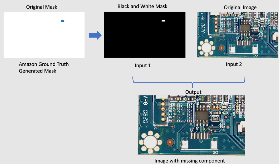
To remove components from the original image, we’re using an open-source PyTorch model called LaMa from LaMa: Resolution-robust Large Mask Inpainting with Fourier Convolutions. It’s a resolution-robust large mask in-painting model with Fourier convolutions developed by Samsung AI. The inputs for the model are an image and a black and white mask and the output is an image with the objects inside the mask removed. We use Amazon SageMaker Ground Truth to create the original mask, and then transform it to a black and white mask as required. The LaMa model application is demonstrated as following:

4.3.2 Introducing Amazon SageMaker Asynchronous inference
Amazon SageMaker Asynchronous Inference is a new inference option in Amazon SageMaker that queues incoming requests and processes them asynchronously. Asynchronous inference enables users to save on costs by autoscaling the instance count to zero when there are no requests to process. This means that you only pay when your endpoint is processing requests. The new asynchronous inference option is ideal for workloads where the request sizes are large (up to 1GB) and inference processing times are in the order of minutes. The code to deploy and invoke the endpoint is here.
4.3.3 Endpoint deployment
To deploy the asynchronous endpoint, first we must get the IAM role and set up some environment variables.
from sagemaker import get_execution_role
from sagemaker.pytorch import PyTorchModel
import boto3

role = get_execution_role()
env = dict()
env['TS_MAX_REQUEST_SIZE'] = '1000000000'
env['TS_MAX_RESPONSE_SIZE'] = '1000000000'
env['TS_DEFAULT_RESPONSE_TIMEOUT'] = '1000000'
env['DEFAULT_WORKERS_PER_MODEL'] = '1'
As we mentioned before, we’re using open source PyTorch model LaMa: Resolution-robust Large Mask Inpainting with Fourier Convolutions and the pre-trained model has been uploaded to s3://qualityinspection/model/big-lama.tar.gz. The image_uri points to a docker container with the required framework and python versions.
model = PyTorchModel(
    entry_point="./inference_defect_gen.py",
    role=role,
    source_dir = './',
    model_data='s3://qualityinspection/model/big-lama.tar.gz',
    image_uri = '763104351884.dkr.ecr.us-west-2.amazonaws.com/pytorch-inference:1.11.0-gpu-py38-cu113-ubuntu20.04-sagemaker',
    framework_version="1.7.1",
    py_version="py3",
    env = env,
    model_server_workers=1
)
Then, we must specify additional asynchronous inference specific configuration parameters while creating the endpoint configuration.
from sagemaker.async_inference.async_inference_config import AsyncInferenceConfig
bucket = 'qualityinspection'
prefix = 'async-endpoint'
async_config = AsyncInferenceConfig(output_path=f"s3://{bucket}/{prefix}/output",max_concurrent_invocations_per_instance=10)
Next, we deploy the endpoint on a ml.g4dn.xlarge instance by running the following code:
predictor = model.deploy(
    initial_instance_count=1,
    instance_type='ml.g4dn.xlarge',
    model_server_workers=1,
    async_inference_config=async_config
)
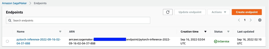
After approximately 6-8 minutes, the endpoint is created successfully, and it will show up in the SageMaker console.

4.3.4 Invoke the endpoint
Next, we use the input txt file we generated earlier as the input of the endpoint and invoke the endpoint using the following code:
import boto3
runtime= boto3.client('runtime.sagemaker')
response = runtime.invoke_endpoint_async(EndpointName='pytorch-inference-2022-09-16-02-04-37-888',
                                   InputLocation='s3://qualityinspection/input/input.txt')
The above command will finish execution immediately. However, the inference will continue for several minutes until it completes all of the tasks and returns all of the outputs in the S3 bucket.
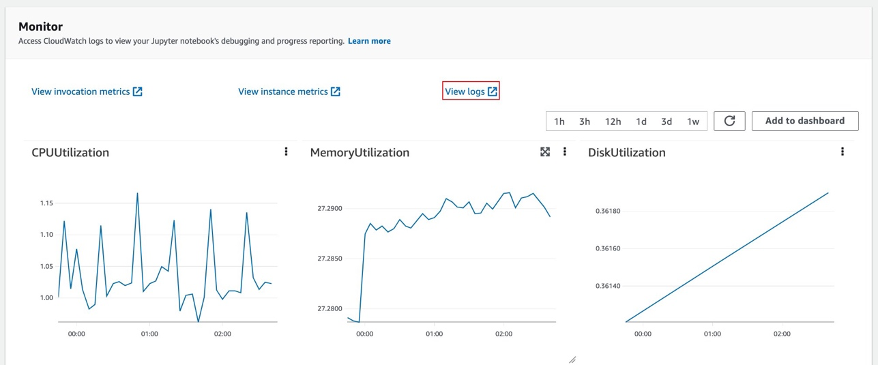
4.3.5 Check the inference result of the endpoint
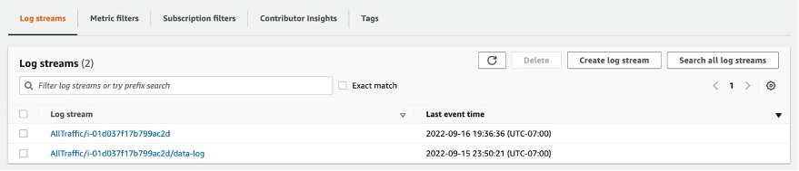
After you select the endpoint, you’ll see the Monitor session. Select ‘View logs’ to check the inference results in the console.

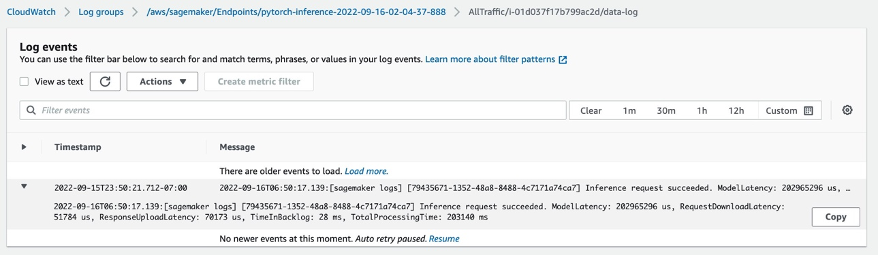
Two log records will show up in Log streams. The one named data-log will show the final inference result, while the other log record will show the details of the inference, which is usually used for debug purposes.

If the inference request succeeds, then you’ll see the message: Inference request succeeded.in the data-log and also get information of the total model latency, total process time, etc. in the message. If the inference fails, then check the other log to debug. You can also check the result by polling the status of the inference request. Learn more about the Amazon SageMaker Asynchronous inference here.

4.3.6 Generating synthetic defects with missing components using the endpoint
We’ll complete four tasks in the endpoint:
- The Lookout for Vision anomaly localization service requires one defect per image in the training dataset to optimize model performance. Therefore, we must separate the masks for different defects in the endpoint by color filtering.

- Split train/test dataset to satisfy the following requirement:
- at least 10 normal images and 10 anomalies for train dataset
- one defect/image in train dataset
- at least 10 normal images and 10 anomalies for test dataset
- multiple defects per image is allowed for the test dataset
- Generate synthetic defects and upload them to the target S3 locations.
We generate one defect per image and more than 20 defects per class for train dataset, as well as 1-3 defects per image and more than 20 defects per class for the test dataset.
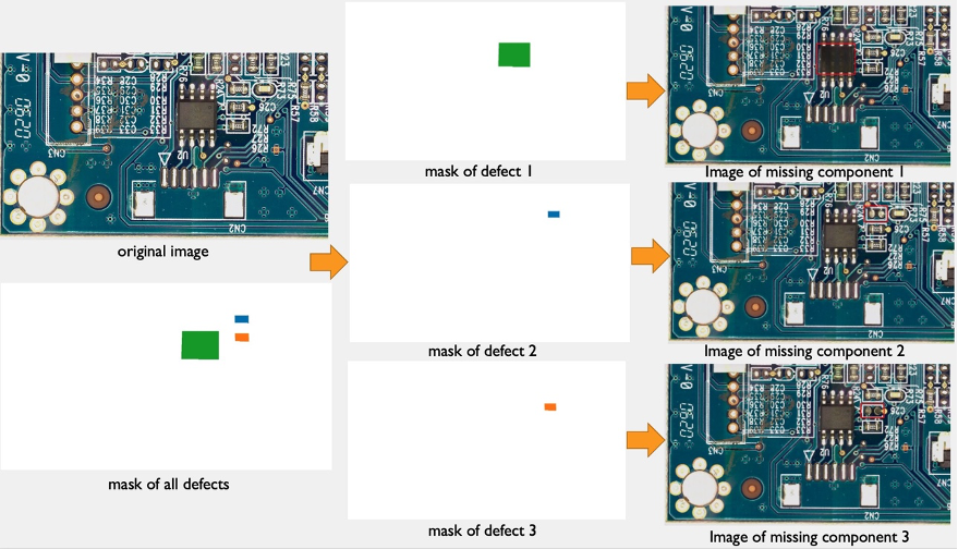
The following is an example of the source image and its synthetic defects with three components: IC, resistor1, and resistor 2 missing.
original image

40_im_mask_IC_resistor1_resistor2.jpg (the defect name indicates the missing components)
- Generate manifest files for train/test dataset recording all of the above information.
Finally, we’ll generate train/test manifests to record information, such as synthetic defect S3 location, mask S3 location, defect class, mask color, etc.
The following are sample json lines for an anomaly and a normal image in the manifest.
For anomaly:
{"source-ref": "s3://qualityinspection/synthetic_defect/anomaly/train/6_im_mask_IC.jpg", "auto-label": 11, "auto-label-metadata": {"class-name": "anomaly", "type": "groundtruth/image-classification"}, "anomaly-mask-ref": "s3://qualityinspection/synthetic_defect/mask/MixMask/mask_IC.png", "anomaly-mask-ref-metadata": {"internal-color-map": {"0": {"class-name": "IC", "hex-color": "#2ca02c", "confidence": 0}}, "type": "groundtruth/semantic-segmentation"}}
For normal image:
{"source-ref": "s3://qualityinspection/synthetic_defect/normal/train/25_im.jpg", "auto-label": 12, "auto-label-metadata": {"class-name": "normal", "type": "groundtruth/image-classification"}}
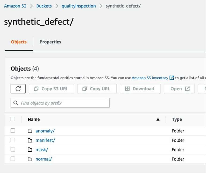
4.3.7 Amazon S3 folder structure
The input and output of the endpoint are stored in the target S3 bucket in the following structure:


5 Lookout for Vision model training and result
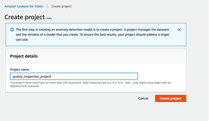
5.1 Set up a project, upload dataset, and start model training.
- First, you can go to Lookout for Vision from the AWS Console and create a project.

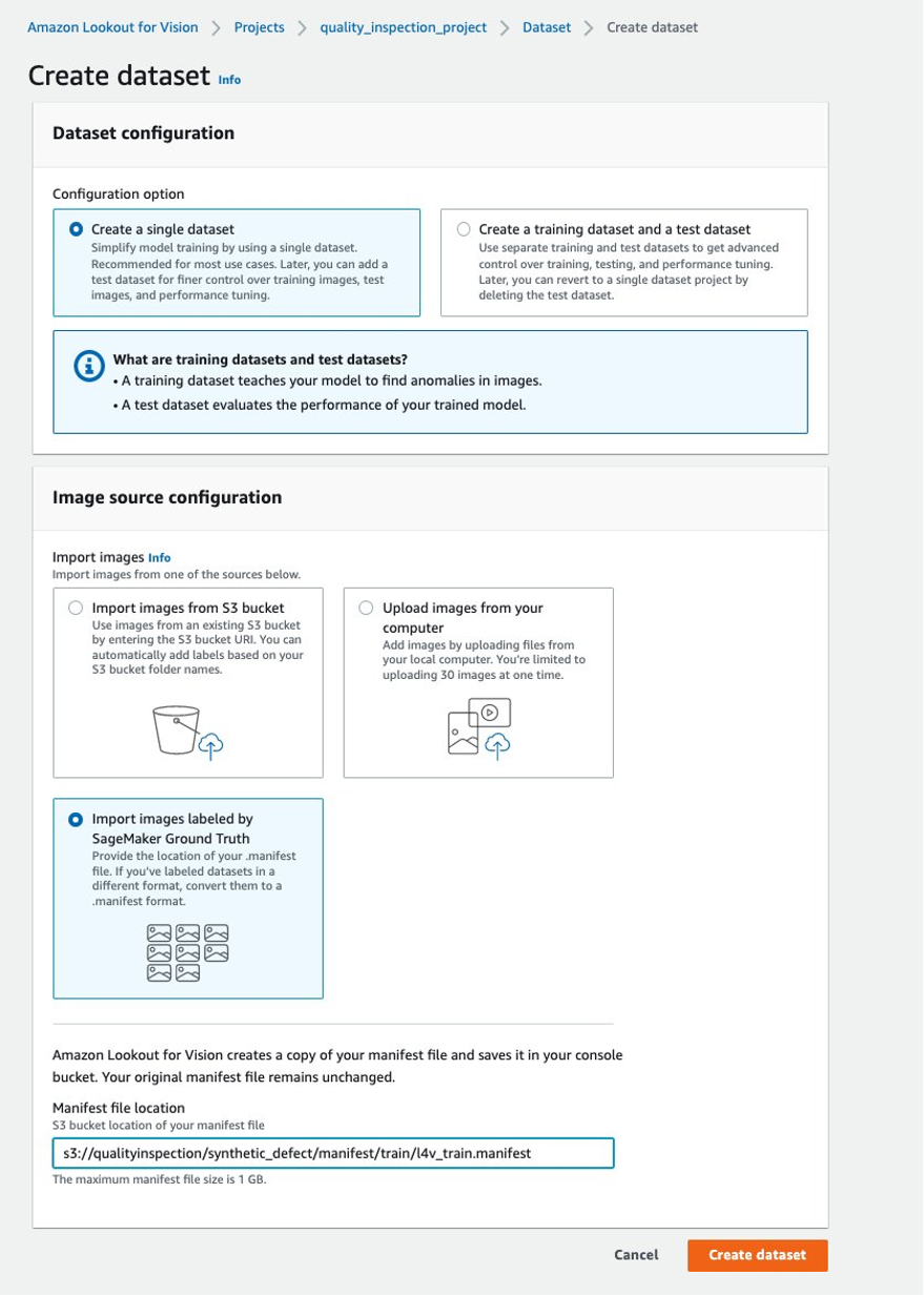
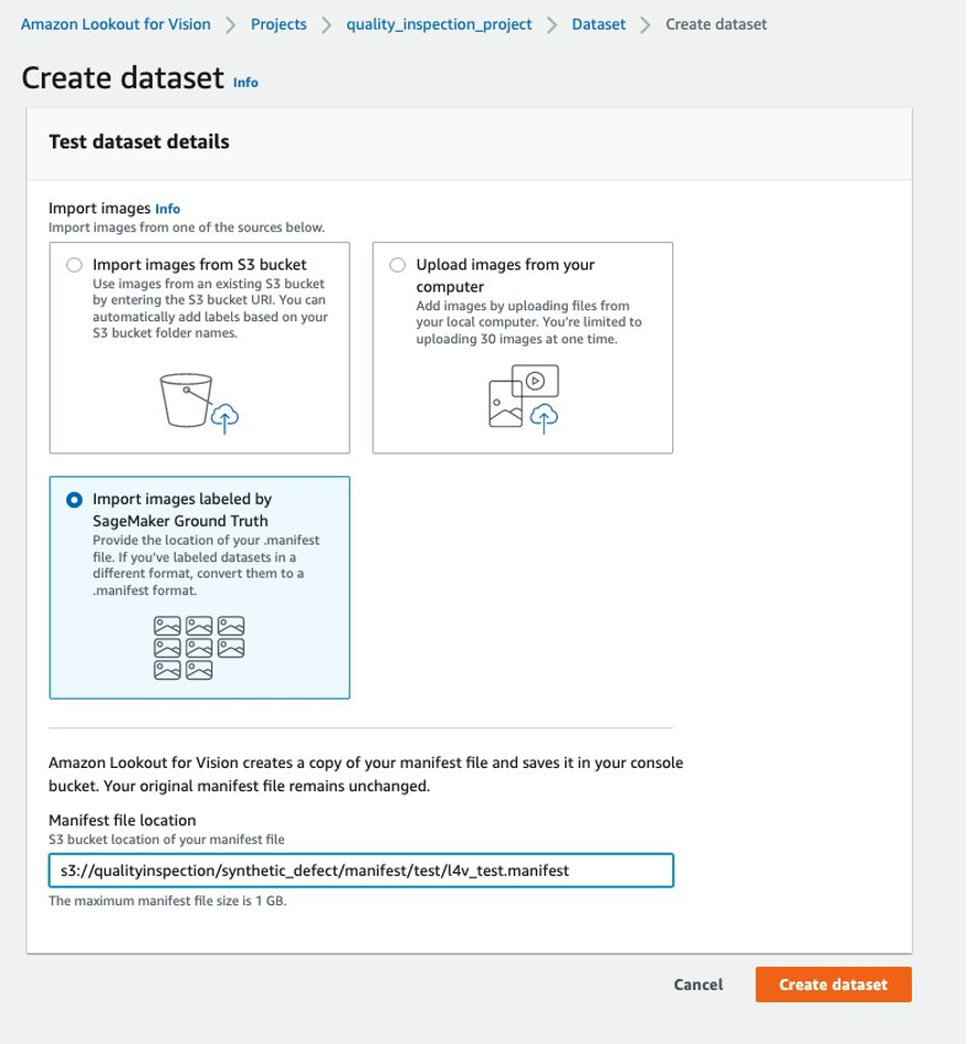
- Then, you can create a training dataset by choosing Import images labeled by SageMaker Ground Truth and give the Amazon S3 location of the train dataset manifest generated by the SageMaker endpoint.

- Next, you can create a test dataset by choosing Import images labeled by SageMaker Ground Truth again, and give the Amazon S3 location of the test dataset manifest generated by the SageMaker endpoint.

…….
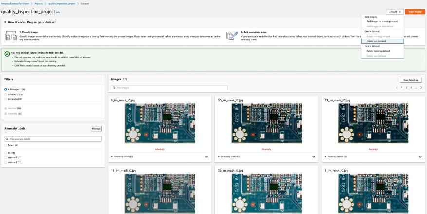
…. - After the train and test datasets are uploaded successfully, you can select the Train model button at the top right corner to trigger the anomaly localization model training.
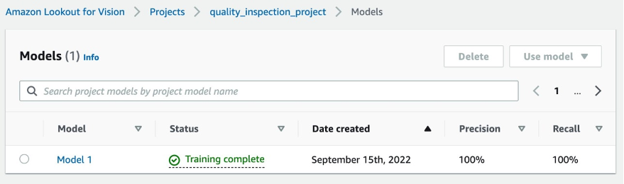
…… - In our experiment, the model took slightly longer than one hour to complete training. When the status shows training complete, you can select the model link to check the result.
….

5.2 Model training result
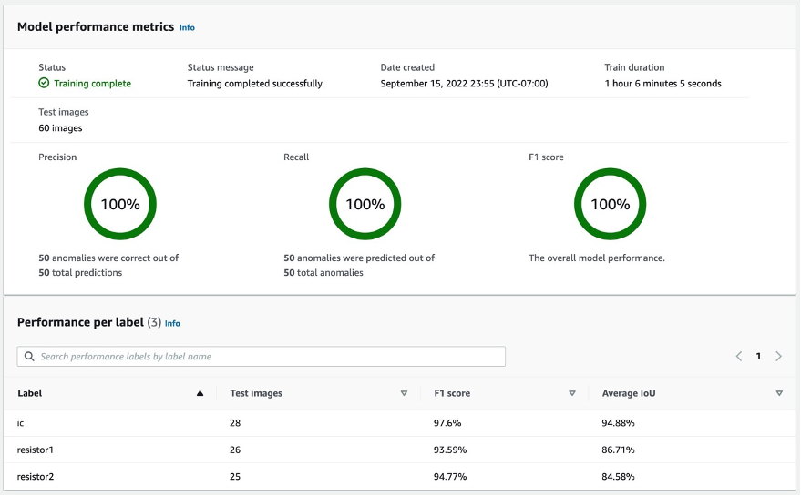
5.2.1 Model performance metrics
After selecting at the Model 1 as shown above, we can see from the 100% Precision, 100% Recall, and 100% F1 score that the model performance is quite good. We can also check the performance per label (missing component), and we’ll be happy to find that all three labels’ F1 scores are above 93%, and the Average IoUs are above 85%. This result is satisfying for this small dataset that we demonstrated in the post.

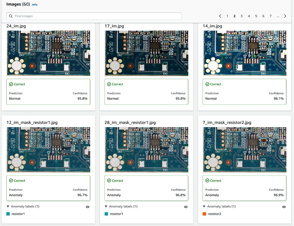
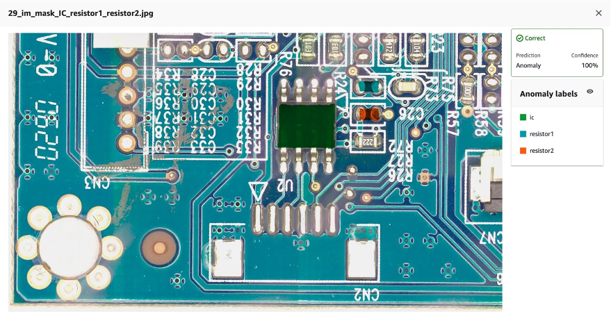
5.2.2 Visualization of synthetic defects detection in the test dataset.
As the following image shows, each image will be defected as an normal or anomaly label with a confidence score. If it’s an anomaly, then it will show a mask over the abnormal area in the image with a different color for each defect type.

The following is an example of combined missing components (three defects in this case) in the test dataset:

Next you can compile and package the model as an AWS IoT Greengrass component following the instructions in this post, Identify the location of anomalies using Amazon Lookout for Vision at the edge without using a GPU, and run inferences on the model.
6. Test the Lookout for Vision model trained on synthetic data against real defects
To test if the model trained on the synthetic defect can perform well against real defects, we picked a dataset (aliens-dataset) from here to run an experiment.
First, we compare the generated synthetic defect and the real defect. The left image is a real defect with a missing head, and the right image is a generated defect with the head removed using an ML model.
 Real defect |  Synthetic defect |
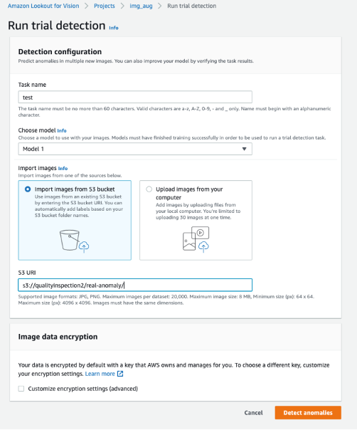
Second, we use the trial detections in Lookout for Vision to test the model against the real defect. You can either save the test images in the S3 bucket and import them from Amazon S3 or upload images from your computer. Then, select Detect anomalies to run the detection.

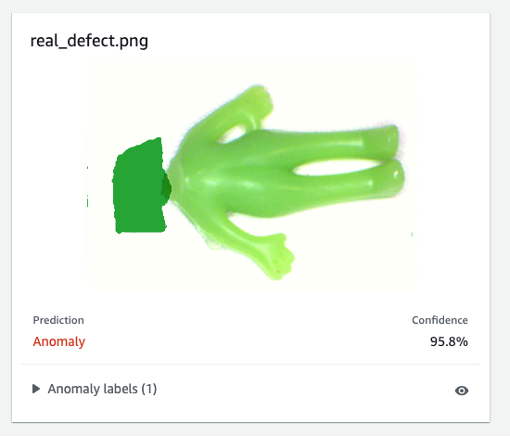
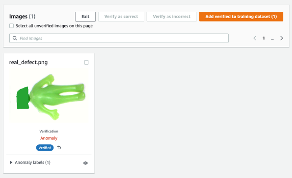
Finally, you can see the prediction result of the real defect. The model trained on synthetic defects can defect the real defect accurately in this experiment.

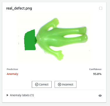
The model trained on synthetic defects may not always perform well on real defects, especially circuit boards which are much more complicated than this sample dataset. If you want to retrain the model with real defects, then you can select the orange button labeled Verify machine predictions in the upper right corner of the prediction result, and then check it as Correct or Incorrect.

Then you can add the verified image and label to the training dataset by selecting the orange button in the upper right corner to enhance model performance.

7. Cost estimation
This image augmentation pipeline for Lookout for Vision is very cost-effective. In the example shown above, Amazon SageMaker Ground Truth Labeling, Amazon SageMaker notebook, and SageMaker asynchronous endpoint deployment and inference only cost a few dollars. For Lookout for Vision service, you pay only for what you use. There are three components that determine your bill: charges for training the model (training hours), charges for detecting anomalies on the cloud (cloud inference hours), and/or charges for detecting anomalies on the edge (edge inference units). In our experiment, the Lookout for Vision model took slightly longer than one hour to complete training, and it cost $2.00 per training hour. Furthermore, you can use the trained model for inference on the cloud or on the edge with the price listed here.
8. Clean up
To avoid incurring unnecessary charges, use the Console to delete the endpoints and resources that you created while running the exercises in the post.
- Open the SageMaker console and delete the following resources:
- The endpoint. Deleting the endpoint also deletes the ML compute instance or instances that support it.
- Under Inference, choose Endpoints.
- Choose the endpoint that you created in the example, choose Actions, and then choose Delete.
- The endpoint configuration.
- Under Inference, choose Endpoint configurations.
- Choose the endpoint configuration that you created in the example, choose Actions, and then choose Delete.
- The model.
- Under Inference, choose Models.
- Choose the model that you created in the example, choose Actions, and then choose Delete.
- The notebook instance. Before deleting the notebook instance, stop it.
- Under Notebook, choose Notebook instances.
- Choose the notebook instance that you created in the example, choose Actions, and then choose Stop. The notebook instance takes several minutes to stop. When the Status changes to Stopped, move on to the next step.
- Choose Actions, and then choose Delete.
- Open the Amazon S3 console, and then delete the bucket that you created for storing model artifacts and the training dataset.
- Open the Amazon CloudWatch console, and then delete all of the log groups that have names starting with
/aws/sagemaker/.
You can also delete the endpoint from SageMaker notebook by running the following code:
import boto3
sm_boto3 = boto3.client("sagemaker")
sm_boto3.delete_endpoint(EndpointName='endpoint name')
9. Conclusion
In this post, we demonstrated how to annotate synthetic defect masks using Amazon SageMaker Ground Truth, how to use different image augmentation techniques to transform one normal image to the desired number of normal images, create an asynchronous SageMaker endpoint and prepare the input file for the endpoint, as well as invoke the endpoint. At last, we demonstrated how to use the train/test manifest to train a Lookout for Vision anomaly localization model. This proposed pipeline can be extended to other ML models to generate synthetic defects, and all you need to do is to customize the model and inference code in the SageMaker endpoint.
Start by exploring Lookout for Vision for automated quality inspection here.
About the Authors
 Kara Yang is a Data Scientist at AWS Professional Services. She is passionate about helping customers achieve their business goals with AWS cloud services and has helped organizations build end to end AI/ML solutions across multiple industries such as manufacturing, automotive, environmental sustainability and aerospace.
 Octavi Obiols-Sales is a computational scientist specialized in deep learning (DL) and machine learning certified as an associate solutions architect. With extensive knowledge in both the cloud and the edge, he helps to accelerate business outcomes through building end-to-end AI solutions. Octavi earned his PhD in computational science at the University of California, Irvine, where he pushed the state-of-the-art in DL+HPC algorithms.
 Fabian Benitez-Quiroz is a IoT Edge Data Scientist in AWS Professional Services. He holds a PhD in Computer Vision and Pattern Recognition from The Ohio State University. Fabian is involved in helping customers run their Machine Learning models with low latency on IoT devices and in the cloud.
 Manish Talreja is a Principal Product Manager for IoT Solutions at AWS. He is passionate about helping customers build innovative solutions using AWS IoT and ML services in the cloud and at the edge.
Yuxin Yang is an AI/ML architect at AWS, certified in the AWS Machine Learning Specialty. She enables customers to accelerate their outcomes through building end-to-end AI/ML solutions, including predictive maintenance, computer vision and reinforcement learning. Yuxin earned her MS from Stanford University, where she focused on deep learning and big data analytics.
 Yingmao Timothy Li is a Data Scientist with AWS. He has joined AWS 11 months ago and he works with a broad range of services and machine learning technologies to build solutions for a diverse set of customers. He holds a Ph.D in Electrical Engineering. In his spare time, He enjoys outdoor games, car racing, swimming, and flying a piper cub to cross country and explore the sky.


 Kara Yang is a Data Scientist at AWS Professional Services. She is passionate about helping customers achieve their business goals with AWS cloud services and has helped organizations build end to end AI/ML solutions across multiple industries such as manufacturing, automotive, environmental sustainability and aerospace.
 Octavi Obiols-Sales is a computational scientist specialized in deep learning (DL) and machine learning certified as an associate solutions architect. With extensive knowledge in both the cloud and the edge, he helps to accelerate business outcomes through building end-to-end AI solutions. Octavi earned his PhD in computational science at the University of California, Irvine, where he pushed the state-of-the-art in DL+HPC algorithms.
 Yuxin Yang is an AI/ML architect at AWS, certified in the AWS Machine Learning Specialty. She enables customers to accelerate their outcomes through building end-to-end AI/ML solutions, including predictive maintenance, computer vision and reinforcement learning. Yuxin earned her MS from Stanford University, where she focused on deep learning and big data analytics.
 Yingmao Timothy Li is a Data Scientist with AWS. He has joined AWS 11 months ago and he works with a broad range of services and machine learning technologies to build solutions for a diverse set of customers. He holds a Ph.D in Electrical Engineering. In his spare time, He enjoys outdoor games, car racing, swimming, and flying a piper cub to cross country and explore the sky.