
As global temperatures rise, wildfires around the world are becoming more frequent and more dangerous. Their effects are felt by many communities as people evacuate their homes or suffer harm even from proximity to the fire and smoke.
As part of Google’s mission to help people access trusted information in critical moments, we use satellite imagery and machine learning (ML) to track wildfires and inform affected communities. Our wildfire tracker was recently expanded. It provides updated fire boundary information every 10–15 minutes, is more accurate than similar satellite products, and improves on our previous work. These boundaries are shown for large fires in the continental US, Mexico, and most of Canada and Australia. They are displayed, with additional information from local authorities, on Google Search and Google Maps, allowing people to keep safe and stay informed about potential dangers near them, their homes or loved ones.
 |
| Real-time boundary tracking of the 2021-2022 Wrattonbully bushfire, shown as a red polygon in Google Maps. |
Inputs
Wildfire boundary tracking requires balancing spatial resolution and update frequency. The most scalable method to obtain frequent boundary updates is to use geostationary satellites, i.e., satellites that orbit the earth once every 24 hours. These satellites remain at a fixed point above Earth, providing continual coverage of the area surrounding that point. Specifically, our wildfire tracker models use the GOES-16 and GOES-18 satellites to cover North America, and the Himawari-9 and GK2A satellites to cover Australia. These provide continent-scale images every 10 minutes. The spatial resolution is 2km at nadir (the point directly below the satellite), and lower as one moves away from nadir. The goal here is to provide people with warnings as soon as possible, and refer them to authoritative sources for spatially precise, on-the-ground data, as necessary.
 |
| Smoke plumes obscuring the 2018 Camp Fire in California. [Image from NASA Worldview] |
Determining the precise extent of a wildfire is nontrivial, since fires emit massive smoke plumes, which can spread far from the burn area and obscure the flames. Clouds and other meteorological phenomena further obscure the underlying fire. To overcome these challenges, it is common to rely on infrared (IR) frequencies, particularly in the 3–4 μm wavelength range. This is because wildfires (and similar hot surfaces) radiate considerably at this frequency band, and these emissions diffract with relatively minor distortions through smoke and other particulates in the atmosphere. This is illustrated in the figure below, which shows a multispectral image of a wildfire in Australia. The visible channels (blue, green, and red) mostly show the triangular smoke plume, while the 3.85 μm IR channel shows the ring-shaped burn pattern of the fire itself. Even with the added information from the IR bands, however, determining the exact extent of the fire remains challenging, as the fire has variable emission strength, and multiple other phenomena emit or reflect IR radiation.
 |
| Himawari-8 hyperspectral image of a wildfire. Note the smoke plume in the visible channels (blue, green, and red), and the ring indicating the current burn area in the 3.85μm band. |
Model
Prior work on fire detection from satellite imagery is typically based on physics-based algorithms for identifying hotspots from multispectral imagery. For example, the National Oceanic and Atmospheric Administration (NOAA) fire product identifies potential wildfire pixels in each of the GOES satellites, primarily by relying on the 3.9 μm and 11.2 μm frequencies (with auxiliary information from two other frequency bands).
In our wildfire tracker, the model is trained on all satellite inputs, allowing it to learn the relative importance of different frequency bands. The model receives a sequence of the three most recent images from each band so as to compensate for temporary obstructions such as cloud cover. Additionally, the model receives inputs from two geostationary satellites, achieving a super-resolution effect whereby the detection accuracy improves upon the pixel size of either satellite. In North America, we also supply the aforementioned NOAA fire product as input. Finally, we compute the relative angles of the sun and the satellites, and provide these as additional input to the model.
All inputs are resampled to a uniform 1 km–square grid and fed into a convolutional neural network (CNN). We experimented with several architectures and settled on a CNN followed by a 1×1 convolutional layer to yield separate classification heads for fire and cloud pixels (shown below). The number of layers and their sizes are hyperparameters, which are optimized separately for Australia and North America. When a pixel is identified as a cloud, we override any fire detection since heavy clouds obscure underlying fires. Even so, separating the cloud classification task improves the performance of fire detection as we incentivize the system to better identify these edge cases.
 |
| CNN architecture for the Australia model; a similar architecture was used for North America. Adding a cloud classification head improves fire classification performance. |
To train the network, we used thermal anomalies data from the MODIS and VIIRS polar-orbiting satellites as labels. MODIS and VIIRS have higher spatial accuracy (750–1000 meters) than the geostationary satellites we use as inputs. However, they cover a given location only once every few hours, which occasionally causes them to miss rapidly-advancing fires. Therefore, we use MODIS and VIIRS to construct a training set, but at inference time we rely on the high-frequency imagery from geostationary satellites.
Even when limiting attention to active fires, most pixels in an image are not currently burning. To reduce the model’s bias towards non-burning pixels, we upsampled fire pixels in the training set and applied focal loss to encourage improvements in the rare misclassified fire pixels.
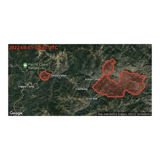
 |
| The progressing boundary of the 2022 McKinney fire, and a smaller nearby fire. |
Evaluation
High-resolution fire signals from polar-orbiting satellites are a plentiful source for training data. However, such satellites use sensors that are similar to geostationary satellites, which increases the risk of systemic labeling errors (e.g., cloud-related misdetections) being incorporated into the model. To evaluate our wildfire tracker model without such bias, we compared it against fire scars (i.e., the shape of the total burnt area) measured by local authorities. Fire scars are obtained after a fire has been contained and are more reliable than real-time fire detection techniques. We compare each fire scar to the union of all fire pixels detected in real time during the wildfire to obtain an image such as the one shown below. In this image, green represents correctly identified burn areas (true positive), yellow represents unburned areas detected as burn areas (false positive), and red represents burn areas that were not detected (false negative).
 |
| Example evaluation for a single fire. Pixel size is 1km x 1km. |
We compare our models to official fire scars using the precision and recall metrics. To quantify the spatial severity of classification errors, we take the maximum distance between a false positive or false negative pixel and the nearest true positive fire pixel. We then average each metric across all fires. The results of the evaluation are summarized below. Most severe misdetections were found to be a result of errors in the official data, such as a missing scar for a nearby fire.
 |
| Test set metrics comparing our models to official fire scars. |
We performed two additional experiments on wildfires in the United States (see table below). First, we evaluated an earlier model that relies only on NOAA’s GOES-16 and GOES-17 fire products. Our model outperforms this approach in all metrics considered, demonstrating that the raw satellite measurements can be used to enhance the existing NOAA fire product.
Next, we collected a new test set consisting of all large fires in the United States in 2022. This test set was not available during training because the model launched before the fire season began. Evaluating the performance on this test set shows performance in line with expectations from the original test set.
 |
| Comparison between models on fires in the United States. |
Conclusion
Boundary tracking is part of Google’s wider commitment to bring accurate and up-to-date information to people in critical moments. This demonstrates how we use satellite imagery and ML to track wildfires, and provide real time support to affected people in times of crisis. In the future, we plan to keep improving the quality of our wildfire boundary tracking, to expand this service to more countries and continue our work helping fire authorities access critical information in real time.
Acknowledgements
This work is a collaboration between teams from Google Research, Google Maps and Crisis Response, with support from our partnerships and policy teams. We would also like to thank the fire authorities whom we partner with around the world.