BigQuery data canvas, a Gemini in BigQuery feature, is a revolutionary data analytics tool that simplifies the entire data analysis journey — from data discovery and preparation to analysis, visualization, and collaboration — all in one place, all within BigQuery. BigQuery data canvas leverages natural language processing to let you can ask questions about your data in plain English and various other languages. This intuitive approach eliminates the need to build out complex SQL queries, making data analysis accessible to both technical and non-technical users. With data canvas, you can explore, transform, and visualize your BigQuery data without ever leaving the environment where your data resides.
In this blog, we present an overview of BigQuery data canvas and a technical walkthrough of a real-world example using the public github_repos dataset. This dataset contains over 3TB of activity from 3M+ open-source repositories. We’ll explore how to answer questions such as:
How many commits were made to a specific repository in a year?
Who authored the most repositories in a given year?
How many non-authored commits were applied over time?
Which users contributed to a specific file at a specific time?
You’ll see how data canvas handles complex SQL tasks like joining tables, unnesting fields, converting timestamps, and extracting specific data elements – all from your natural language prompts. We’ll even demonstrate how to generate insightful visualizations and summaries with a single click.
BigQuery data canvas at a glance
At its core, BigQuery data canvas provides three key areas of functionality: You can use it to help you find data, generate SQL, and generate insights.
The three aspects of BigQuery data canvas
1. Find data
Use data canvas to find data in BigQuery with a quick keyword search or a natural-language text prompt.
Start your analysis journey in BigQuery’s data canvas powered by Gemini
2. Generate SQL
You can also use BigQuery data canvas to write SQL code for you, also with Gemini-powered natural language prompts.
Create SQL queries for the chosen table using simple English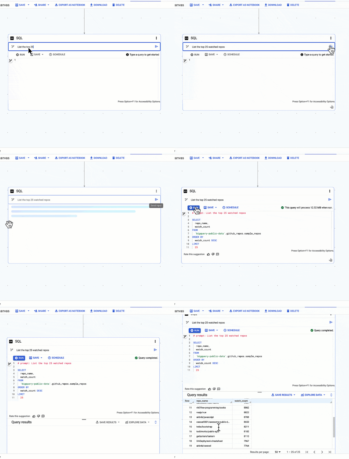
3. Create insights
Finally, discover insights hidden within your data with a single click! Gemini automatically generates visualizations to help you understand the story your data is telling.
Gemini automatically generates visualizations to help you understand the story your data is telling.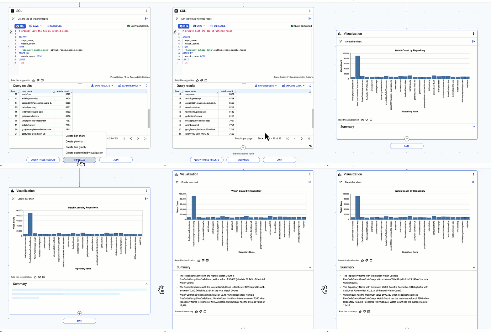
BigQuery data canvas in action
To give you a better sense of how the impact BigQuery data canvas can have in your organization, let’s take an example. Companies of all sizes, from large enterprises to small startups, can benefit from a deeper understanding of their developer team’s productivity. In this technical deep dive, we’ll show you how to use the github_repos public dataset with data canvas to generate valuable insights in a shareable workspace. Through this example, you’ll see how data canvas makes it easy to perform complex queries — allowing you to create SQL that joins and unnests nested fields, converts timestamps, extracts month/year from date fields, and more. With Gemini’s capabilities, you can easily generate these queries and explore your data, with insightful visualizations, all using natural language.
Please note that as with many new AI products and services today, you need strong prompt engineering skills for the successful use of any LLM-enabled application. Many may perceive that out-of-the-box large language models (LLMs) are not good at generating SQL. But in our experience, with the right prompting techniques, Gemini in BigQuery via data canvas can generate complex SQL queries with the context of your data corpus. We see that data canvas determines the sorting, grouping, ordering, limiting the record count and SQL structure based on natural language queries. To learn about engineering prompts for BigQuery data canvas, check out our other blog post, BigQuery BigQuery Data Canvas: Prompting Best Practices.
The github_repos dataset, available in Bigquery Public Datasets, is a 3TB+ dataset that contains activity on 3M+ open-source repositories about commits, watch counts, etc., in multiple tables. For this example, we want to look at Google Cloud Platform repository. As always, ensure you have the proper IAM permissions before getting started. Along with these, ensure you have proper permissions to the data canvas and datasets to run nodes successfully.
Exploring each of the tables within the github_repos dataset is easy to do with data canvas. Here, we compare datasets side-by-side, examine schema, details, and preview data, all in the same panel.
Explore tables side-by-side – examine the schema, view details, and preview data
Once you’ve selected your dataset, you can branch another node to query or join it with another table by hovering at the node’s bottom. Arrows indicate the dataset for the next transformation node. When sharing the canvas, you can name each node for clarity. Options in the top right allow you to delete, debug, duplicate, or execute all of the nodes in a series. You can download results, or export data to Sheets or Looker Studio. You can also rate SQL suggestions, restore prior versions, and view the DAG structure in the navigation panel.
Overview of entire data canvas from end-to-end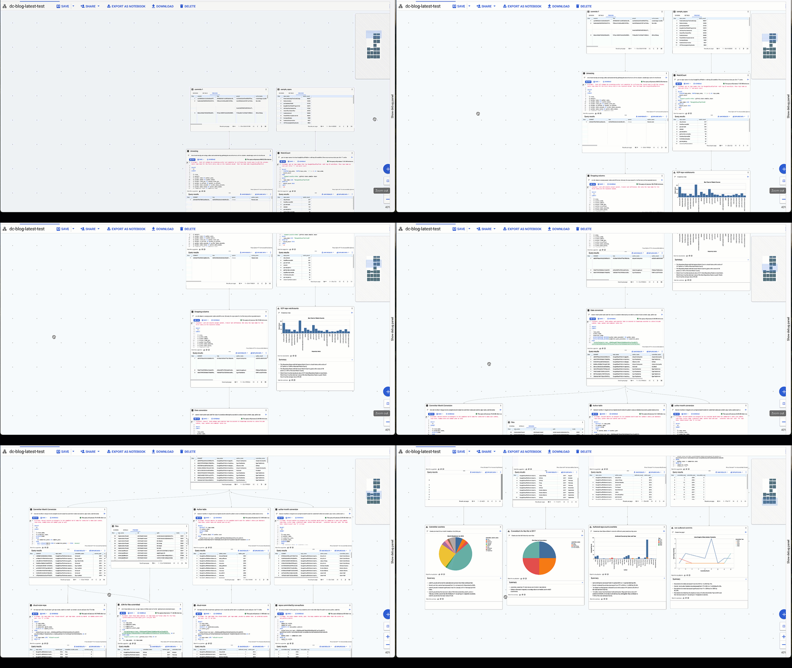
In exploring the github_repos dataset, we look at four different aspects of our data. We’ll look at determining the following:
1) The number of commits made throughout a single year
2) The number of authored repos for a given year
3) How many non-authored commits were applied throughout the years
4) Find the number of commits done by users for a given file at a given time
Below are five major examples of complex SQL queries and transformations generated by the natural language query prompts in this example workflow.
1. Unnest specific columns and find all with Google Cloud Platform in the repo_name
# prompt: list all columns by unnesting author and committer by prefixing the record name to all the columns. match repo name for the first entry only in the repeated column that has name like GoogleCloudPlatform. Make sure to use "%" for like
Generated SQL:
- code_block
- <ListValue: [StructValue([(‘code’, “SELECTrn t1.rnCOMMITrn ,rn t1.tree,rn t1.parent,rn t1.author.name AS author_name,rn t1.author.email AS author_email,rn t1.author.time_sec AS author_time_sec,rn t1.author.tz_offset AS author_tz_offset,rn t1.author.date.seconds AS author_date_seconds,rn t1.author.date.nanos AS author_date_nanos,rn t1.committer.name AS committer_name,rn t1.committer.email AS committer_email,rn t1.committer.time_sec AS committer_time_sec,rn t1.committer.tz_offset AS committer_tz_offset,rn t1.committer.date.seconds AS committer_date_seconds,rn t1.committer.date.nanos AS committer_date_nanos,rn t1.subject,rn t1.message,rn t1.trailer,rn t1.difference,rn t1.difference_truncated,rn t1.repo_name,rn t1.encodingrnFROMrn `bigquery-public-data`.github_repos.commits AS t1rnWHERErn t1.repo_name[rnOFFSETrn (0)] LIKE ‘%GoogleCloudPlatform%'”), (‘language’, ”), (‘caption’, <wagtail.rich_text.RichText object at 0x3e6d6fb6fc10>)])]>
Proper un-nesting of fields under author and committer then filtering down to GoogleCloudPlatform repo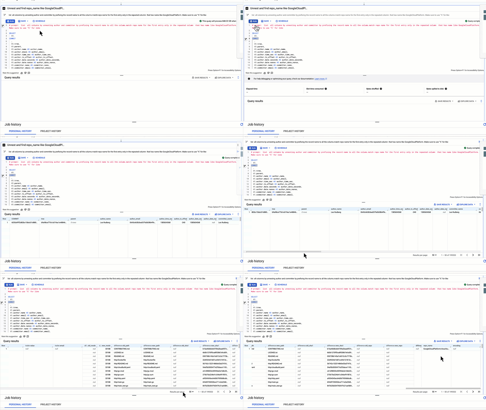
To determine which committers amended a specific file in repositories, we perform a table join to achieve the desired results as in the example below. An option is given at the bottom of each node to query or join the existing table or query results.
2: Inner join of previous query results with github_repos.files table on repo_name
# prompt: Join these data sources on repo name and filter only for the file "python/awwvision/redis/spec.yaml" and year 2017
Generated SQL:
- code_block
- <ListValue: [StructValue([(‘code’, “SELECTrn t1.repo_name,rn t1.committer_name,rn t1.commit_year,rn t1.committer_month_namernFROMrn`carbonfootprint-test._258496aad0f70ded1533d656e2d91ec72ca85379.anon5510948aef153ab43d93ee1c7e056ea8358e1faffbf610cdf152f495f349d3fb` AS t1rnINNER JOINrn `bigquery-public-data`.github_repos.files AS t2rnONrn t1.repo_name = t2.repo_namernWHERErn t2.path = ‘python/awwvision/redis/spec.yaml’rn AND t1.commit_year = 2017″), (‘language’, ”), (‘caption’, <wagtail.rich_text.RichText object at 0x3e6d6fb6f160>)])]>
Table join of query results with github_repos.files table on repo_name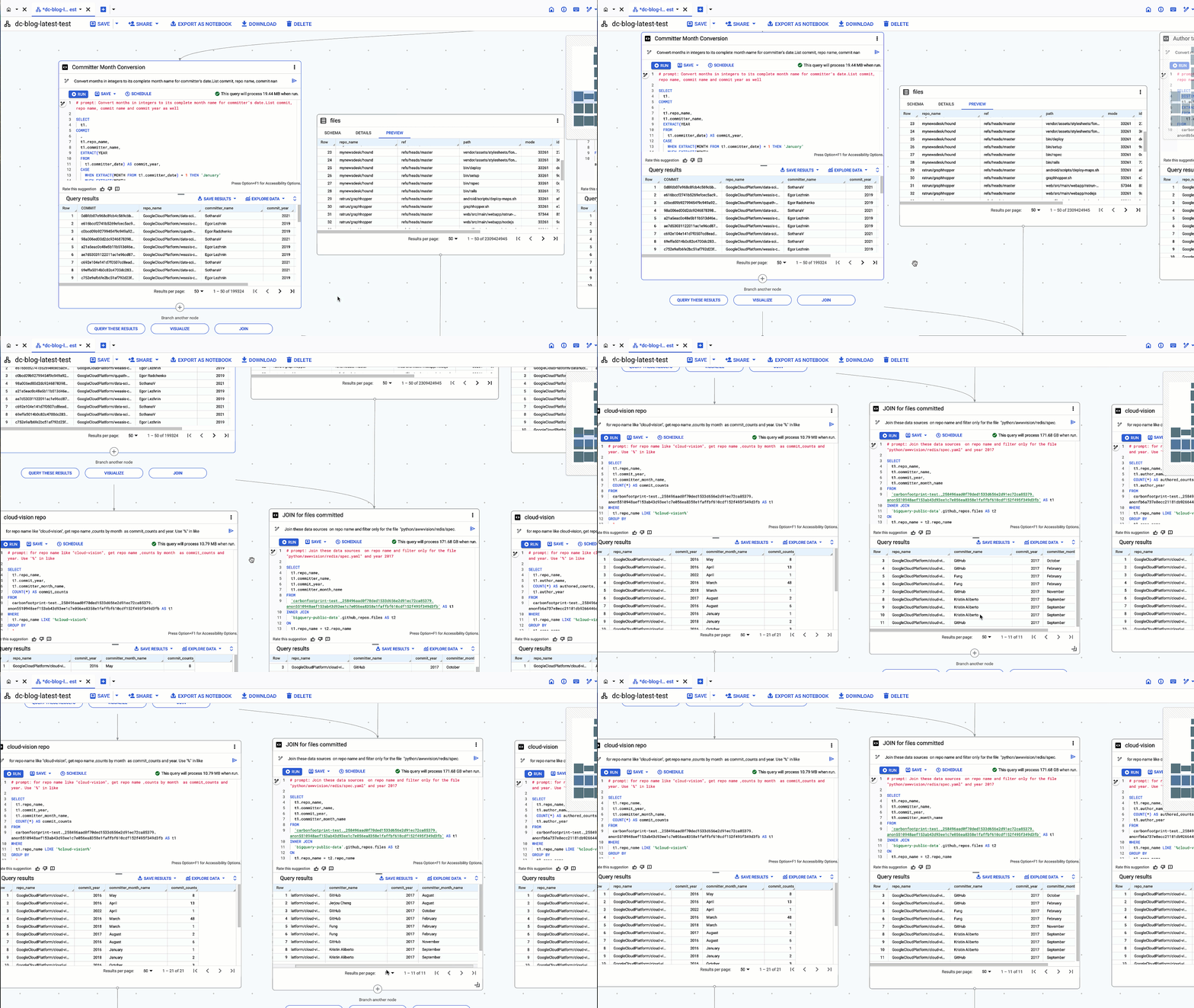
Another prime example of using NL2SQL in data canvas is to convert data types. We need date conversions to convert the epoch time of the author date and committer dates to an actual date. Gemini understands the epoch time unit in seconds and applies the right timestamp and date functions in the right order to convert the dates correctly. We see that activity data in github_repos spans the years 2016 – 2022, which aligns with the results as expected.
3. Date conversion of author date and committer date expressed in seconds
# prompt: convert both author and commiter date in seconds to timestamp seconds to a date. Include commit, repo, author and commiter names too
Generated SQL:
- code_block
- <ListValue: [StructValue([(‘code’, ‘SELECTrnCOMMITrn ,rn repo_name,rn author_name,rn committer_name,rn DATE(TIMESTAMP_SECONDS(author_date_seconds)) AS author_date,rn DATE(TIMESTAMP_SECONDS(committer_date_seconds)) AS committer_daternFROMrn`carbonfootprint-test._258496aad0f70ded1533d656e2d91ec72ca85379.anon5c5de2bd9845a56e6bf97c0ea3e27666c2afa318d8da0a3eb691a76873625eea`’), (‘language’, ”), (‘caption’, <wagtail.rich_text.RichText object at 0x3e6d6fb6f340>)])]>
Author date and committer date correctly converted from epoch time in seconds
Taking it a step further, you can see how well Gemini generates a complex query and figures out the logic based solely on what is asked. In this case, we asked it to extract the month and year from dates and to convert months in integers to the months’ actual names. This is considerably faster than creating the query by hand, and can be easily shared with other members of the team.
4: Extracting month and year from date types and converting months in integers to full month names.
# prompt: Convert months in integers to its complete month name for committer's date. List commit, repo name, author name ,committer name, author date and year , committer date and year for repo like 'cloud-vision’. Use "%" in like
Generated SQL:
- code_block
- <ListValue: [StructValue([(‘code’, “SELECTrn t1.rnCOMMITrn ,rn t1.repo_name,rn t1.author_name,rn t1.committer_name,rn t1.author_date,rn EXTRACT(YEARrn FROMrn t1.committer_date) AS committer_year,rn EXTRACT(MONTHrn FROMrn t1.committer_date) AS committer_month,rn CASErn WHEN EXTRACT(MONTH FROM t1.committer_date) = 1 THEN ‘January’rn WHEN EXTRACT(MONTHrn FROMrn t1.committer_date) = 2 THEN ‘February’rn WHEN EXTRACT(MONTH FROM t1.committer_date) = 3 THEN ‘March’rn WHEN EXTRACT(MONTHrn FROMrn t1.committer_date) = 4 THEN ‘April’rn WHEN EXTRACT(MONTH FROM t1.committer_date) = 5 THEN ‘May’rn WHEN EXTRACT(MONTHrn FROMrn t1.committer_date) = 6 THEN ‘June’rn WHEN EXTRACT(MONTH FROM t1.committer_date) = 7 THEN ‘July’rn WHEN EXTRACT(MONTHrn FROMrn t1.committer_date) = 8 THEN ‘August’rn WHEN EXTRACT(MONTH FROM t1.committer_date) = 9 THEN ‘September’rn WHEN EXTRACT(MONTHrn FROMrn t1.committer_date) = 10 THEN ‘October’rn WHEN EXTRACT(MONTH FROM t1.committer_date) = 11 THEN ‘November’rn WHEN EXTRACT(MONTHrn FROMrn t1.committer_date) = 12 THEN ‘December’rnENDrn AS committer_month_namernFROMrncarbonfootprint-test._258496aad0f70ded1533d656e2d91ec72ca85379.anon8b5e7308ef0b4726721f5682b48ec5c51cd6137e7fae309474de23971464dd33 AS t1rnWHERErn t1.repo_name LIKE ‘%cloud-vision%'”), (‘language’, ”), (‘caption’, <wagtail.rich_text.RichText object at 0x3e6d6fab9d00>)])]>
Conversion of months expressed in integers to full month names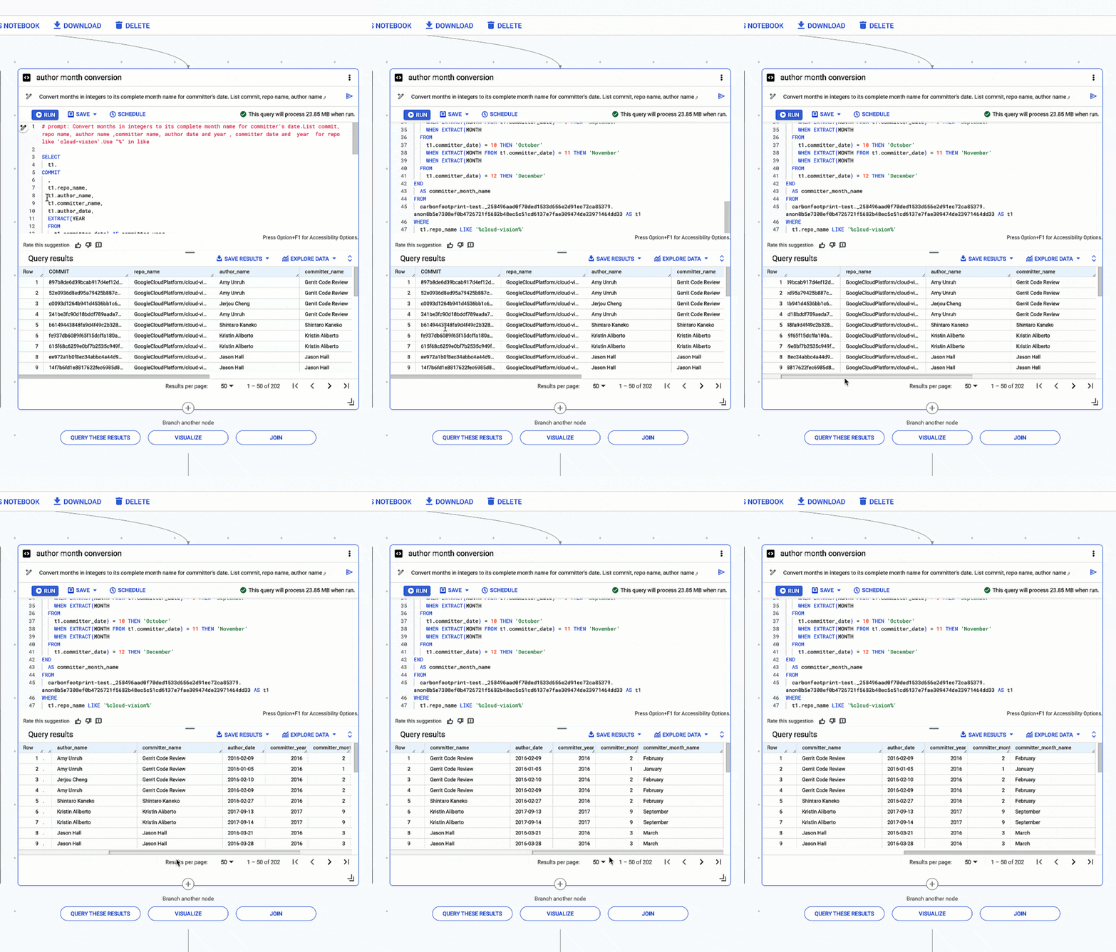
We also demonstrate filtering down data by specifying a specific repo_name and examining the number of commit_counts to this specific repository in a given year. From this, we can use NL2Chart to generate a pie chart. You’ll notice that there’s even an option to generate a gen AI summary for your data. This goes a step further and defines key points of the chart that are not apparent at first glance. Hovering over specific parts of the chart also yields a description with the pointer tooltip. You can export this visualization a png or looker studio or share it with others as well. You can edit chart properties as well as access a JSON output editor by clicking the edit option at the bottom of the node.
5: Generate visualizations and summaries on a specific repo_name
# prompt: for repo name like "cloud-vision", get repo name ,counts by month as commit_counts and year. Use “%" in like
Generated SQL:
- code_block
- <ListValue: [StructValue([(‘code’, “SELECTrn t1.repo_name,rn t1.commit_year,rn t1.committer_month_name,rn COUNT(*) AS commit_countsrnFROMrncarbonfootprint-test._258496aad0f70ded1533d656e2d91ec72ca85379.anon5510948aef153ab43d93ee1c7e056ea8358e1faffbf610cdf152f495f349d3fb AS t1rnWHERErn t1.repo_name LIKE ‘%cloud-vision%’rnGROUP BYrn 1,rn 2,rn 3rnrnrnPrompt: rnCreate pie chart. Show month breakdown for 2016 year.”), (‘language’, ”), (‘caption’, <wagtail.rich_text.RichText object at 0x3e6d6fab9940>)])]>
Resulting visualization:
Resulting pie chart shows the number committers over the period of a year, 2016
Finally, once you’ve completed designing your ETL (Extract, Transform, Load) workflow visually in DAG form with BigQuery data canvas, you can export it to BigQuery Colab Enterprise notebooks, transitioning from a visual format to a coded notebook environment for further analysis or customization. Remember, it’s important to have the right networking parameters set up to connect to a runtime environment, so refer to this reference on Notebooks in BQ Studio.
Streamline data analysis with BigQuery data canvas
When dealing with extensive datasets that span various domains, it can be hard to understand the data for a new project or use case. Using data canvas can streamline this process. By simplifying data analysis through natural language-based SQL generation and visualizations, data canvas can enhance your efficiency and expedite workflows, minimizing repetitive queries and allowing you to schedule automatic data refreshes. BigQuery data canvas is generally available – get started today! And for prompt engineering best practices, be sure to read our companion blog, BigQuery Data Canvas: Prompting Best Practices.
